---
title: "Digital Divide Narrows: Internet Adoption Across Generations"
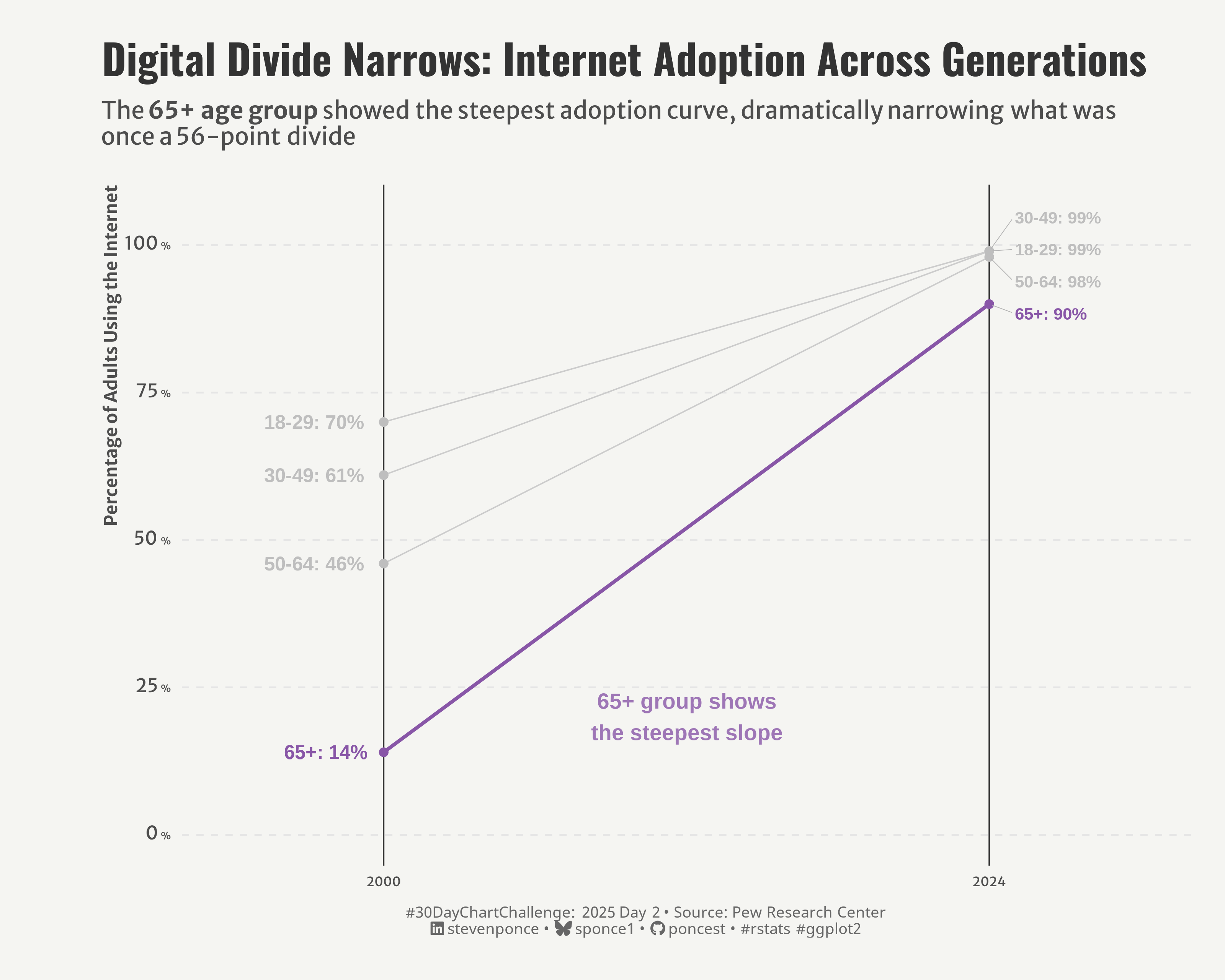
subtitle: "The 65+ age group showed the steepest adoption curve, dramatically narrowing what was once a 56-point divide"
description: "Exploring the dramatic narrowing of the digital divide in the United States from 2000 to 2024, with a focus on how the 65+ age group showed the steepest adoption curve, dramatically closing what was once a significant gap in internet usage between generations."
author: "Steven Ponce"
date: "2025-04-02"
categories: ["30DayChartChallenge", "2025"]
tags: [
"ggplot2",
"slope chart",
"digital divide",
"internet adoption",
"technology trends",
"data journalism",
"generational analysis",
"Pew Research",
"time series",
"social change"
]
image: "thumbnails/30dcc_2025_02.png"
format:
html:
toc: true
toc-depth: 5
code-link: true
code-fold: true
code-tools: true
code-summary: "Show code"
editor_options:
chunk_output_type: inline
execute:
freeze: true
cache: true
error: false
message: false
warning: false
eval: true
# filters:
# - social-share
# share:
# permalink: "https://stevenponce.netlify.app/data_visualizations/30DayChartChallenge/2025/30dcc_2025_02.html"
# description: "The 65+ age group showed the most dramatic internet adoption rate of any generation, rising from just 14% in 2000 to 90% in 2024. This #30DayChartChallenge visualization highlights how seniors closed a once-significant digital divide. #DataViz #rstats"
# twitter: true
# linkedin: true
# email: true
# facebook: false
# reddit: false
# stumble: false
# tumblr: false
# mastodon: true
# bsky: true
---
{#fig-1}
### <mark> **Steps to Create this Graphic** </mark>
#### 1. Load Packages & Setup
```{r}
#| label: load
#| warning: false
#| message: false
#| results: "hide"
## 1. LOAD PACKAGES & SETUP ----
suppressPackageStartupMessages({
pacman::p_load(
  tidyverse,      # Easily Install and Load the 'Tidyverse'
  ggtext,         # Improved Text Rendering Support for 'ggplot2'
  showtext,       # Using Fonts More Easily in R Graphs
  janitor,        # Simple Tools for Examining and Cleaning Dirty Data
  skimr,          # Compact and Flexible Summaries of Data
  scales,         # Scale Functions for Visualization
  lubridate,      # Make Dealing with Dates a Little Easier
  ggrepel,        # Automatically Position Non-Overlapping Text Labels with 'ggplot2'
  camcorder       # Record Your Plot History
)
})

### |- figure size ----
gg_record(
    dir    = here::here("temp_plots"),
    device = "png",
    width  =  10,
    height =  8,
    units  = "in",
    dpi    = 320
)

# Source utility functions
suppressMessages(source(here::here("R/utils/fonts.R")))
source(here::here("R/utils/social_icons.R"))
source(here::here("R/utils/image_utils.R"))
source(here::here("R/themes/base_theme.R"))
```
#### 2. Read in the Data
```{r}
#| label: read
#| include: true
#| eval: true
#| warning: false
internet_raw <- read_delim(
  here::here('data/30DayChartChallenge/2025/internet_use_by_age_data_2024-11-13.csv'),
  skip = 3) |> clean_names() |>
    head(-2)
```
#### 3. Examine the Data
```{r}
#| label: examine
#| include: true
#| eval: true
#| results: 'hide'
#| warning: false
glimpse(internet_raw)
skim(internet_raw)
```
#### 4. Tidy Data
```{r}
#| label: tidy
#| warning: false
### |- Tidy ----
internet_clean <- internet_raw |>
  # Remove whitespace from year and convert to numeric
  mutate(
    year = as.numeric(year),
    across(
      c(ages_18_29, x30_49, x50_64, x65),
      ~ as.numeric(str_remove(., "%")) / 100
    )
  ) |>
  rename(
    "18-29" = ages_18_29,
    "30-49" = x30_49,
    "50-64" = x50_64,
    "65+" = x65
  ) |>
  pivot_longer(
    cols = c("18-29", "30-49", "50-64", "65+"),
    names_to = "age_group",
    values_to = "internet_usage"
  ) |>
  mutate(
    age_group = factor(age_group,
                       levels = c("18-29", "30-49", "50-64", "65+")
    )
  ) |>
  filter(year %in% c(2000, 2024))
```
#### 5. Visualization Parameters
```{r}
#| label: params
#| include: true
#| warning: false
### |- plot aesthetics ----
colors <- get_theme_colors(palette = c(
  "18-29" = "gray",
  "30-49" = "gray",
  "50-64" = "gray",
  "65+" = "#8856a7"
  ))

### |-  titles and caption ----
# text
title_text    <- str_glue("Digital Divide Narrows: Internet Adoption Across Generations")
subtitle_text <- str_glue("The __65+ age group__ showed the steepest adoption curve, dramatically narrowing what was<br>
                          once a 56-point divide")

# Create caption
caption_text <- create_dcc_caption(
  dcc_year = 2025,
  dcc_day = 02,
  source_text =  "Pew Research Center"
)

### |-  fonts ----
setup_fonts()
fonts <- get_font_families()

### |-  plot theme ----

# Start with base theme
base_theme <- create_base_theme(colors)

# Add weekly-specific theme elements
weekly_theme <- extend_weekly_theme(
  base_theme,
  theme(
    # Text styling
    plot.title = element_text(face = "bold", family = fonts$title, size = rel(1.14), margin = margin(b = 10)),
    plot.subtitle = element_text(family = fonts$subtitle, color = colors$text, size = rel(0.78), margin = margin(b = 20)),

    # Axis elements
    axis.title.y = element_text(color = colors$text, size = rel(0.8),
                              hjust = 1, vjust = 0.5, angle = 90),
    axis.title.x = element_blank(),
    axis.text.x = element_text(color = colors$text, size = rel(0.7)),
    axis.text.y = ggtext::element_markdown(),

    # Grid elements
    panel.grid.major = element_blank(),
    panel.grid.minor = element_blank(),

    # Legend elements
    legend.position = "top",
    legend.title = element_text(family = fonts$text, size = rel(0.8)),
    legend.text = element_text(family = fonts$text, size = rel(0.7)),

    # Plot margins
    plot.margin = margin(t = 20, r = 20, b = 20, l = 60),
  )
)

# Set theme
theme_set(weekly_theme)
```
#### 6. Plot
```{r}
#| label: plot
#| warning: false
### |-  Plot ----
p <- ggplot(data = internet_clean) +
  # Geoms
  geom_hline(
    yintercept = seq(0, 1, 0.25),
    color = "gray90",
    linetype = "dashed"
  ) +
  geom_vline(
    xintercept = c(2000, 2024),
    color = '#333333',
    linewidth = 0.4
  ) +
  geom_line(                            # gray lines
    data = internet_clean %>% filter(age_group != "65+"),
    aes(x = year, y = internet_usage, group = age_group),
    color = "gray80",
    linewidth = 0.4
  ) +
  geom_line(                           # selected line
    data = internet_clean %>% filter(age_group == "65+"),
    aes(x = year, y = internet_usage, group = age_group, color = age_group),
    linewidth = 1.0
  ) +
  geom_point(
    aes(x = year, y = internet_usage, color = age_group),
    size = 2
  ) +
  geom_text(                           # 2000 labels
    data = internet_clean %>% filter(year == 2000),
    aes(x = year, y = internet_usage,
        label = paste0(age_group, ": ", percent(internet_usage, accuracy = 1)),
        color = age_group),
    hjust = 1.2,
    fontface = "bold",
    size = 4
  ) +
  geom_text_repel(                     # 2024 labels
    data = internet_clean %>% filter(year == 2024),
    aes(x = year, y = internet_usage,
        label = paste0(age_group, ": ", percent(internet_usage, accuracy = 1)),
        color = age_group),
    hjust = 0,
    direction = "y",
    nudge_x = 1,
    segment.size = 0.2,
    segment.color = "gray70",
    min.segment.length = 0,
    fontface = "bold",
    size = 3.5,
    box.padding = 0.4,
    point.padding = 0.1,
    force = 2
  ) +
  annotate(                           # note
    "text",
    x = 2012,
    y = 0.2,
    label = "65+ group shows\nthe steepest slope",
    color = colors$palette[4],
    fontface = "bold",
    size = 4.5,
    alpha = 0.8
  ) +
  # Scales
  scale_y_continuous(
    limits = c(0, 1.05),
    breaks = c(0, 0.25, 0.50, 0.75, 1.00),
    labels = scales::label_percent(
      suffix = '<span style="font-size:6pt;"> %</span>'
    )
  ) +
  scale_x_continuous(
    breaks = c(2000, 2024),
    labels = c("2000", "2024"),
    limits = c(1992, 2032),
    expand = c(0, 0),
  ) +
  scale_color_manual(
    values = colors$palette,
    guide = "none"
  ) +
  # Labs
  labs(
    title = title_text,
    subtitle = subtitle_text,
    caption = caption_text,
    x = NULL,
    y = "Percentage of Adults Using the Internet"
  ) +
  # Theme
  theme(
    plot.title = element_text(
      size          = rel(1.75),
      family        = fonts$title,
      face          = "bold",
      color         = colors$title,
      margin        = margin(t = 5, b = 5)
    ),
    plot.subtitle   = element_markdown(
      size          = rel(1),
      family        = fonts$subtitle,
      color         = colors$subtitle,
      lineheight    = 1.1,
      margin        = margin(t = 5, b = 20)
    ),
    plot.caption    = element_markdown(
      size          = rel(.65),
      family        = fonts$caption,
      color         = colors$caption,
      lineheight    = 0.65,
      hjust         = 0.5,
      halign        = 0.5,
      margin        = margin(t = 10, b = 5)
    ),
  )
```
#### 7. Save
```{r}
#| label: save
#| warning: false
### |-  plot image ----

save_plot(
  p,
  type = "30daychartchallenge",
  year = 2025,
  day = 02,
  width = 10,
  height = 8
  )
```
#### 8. Session Info
::: {.callout-tip collapse="true"}
##### Expand for Session Info
```{r, echo = FALSE}
#| eval: true
#| warning: false
sessionInfo()
```
:::
#### 9. GitHub Repository
::: {.callout-tip collapse="true"}
##### Expand for GitHub Repo
The complete code for this analysis is available in [`30dcc_2025_02.qmd`](https://github.com/poncest/personal-website/blob/master/data_visualizations/TidyTuesday/2025/30dcc_2025_02.qmd).
For the full repository, [click here](https://github.com/poncest/personal-website/).
:::
#### 10. References
::: {.callout-tip collapse="true"}
##### Expand for References
1. Data Sources:
- Internet, Broadband Fact Sheet: Fact Sheets: Tech Adoption Trends, Pew Research Center, published November 13, 2024 [Internet use by age](https://www.pewresearch.org/internet/fact-sheet/internet-broadband/)
:::
