The Complicated Relationship Between Assists and Turnovers

NBA 2023-24 Season: Correlation = 0.64. Playmakers who create more assists also tend to commit more turnovers

30DayChartChallenge

2025

Exploring the nuanced relationship between playmaking and ball security in the NBA, this visualization reveals how elite players navigate the trade-off between generating assists and limiting turnovers.

Author

Steven Ponce

Published

April 15, 2025

Figure 1: Scatter plot showing NBA 2023-24 season data comparing assists versus turnovers per 36 minutes (correlation = 0.64). Players are divided into four categories: Efficient Playmakers, High-Risk Playmakers, Low-Usage Ball Handlers, and Turnover-Prone. Key players like Haliburton, Wembanyama, and James are labeled, illustrating the complicated relationship between playmaking and ball security.

Steps to Create this Graphic

1. Load Packages & Setup

Show code

## 1. LOAD PACKAGES & SETUP ----
suppressPackageStartupMessages({
pacman::p_load(
  tidyverse,      # Easily Install and Load the 'Tidyverse'
  ggtext,         # Improved Text Rendering Support for 'ggplot2'
  showtext,       # Using Fonts More Easily in R Graphs
  janitor,        # Simple Tools for Examining and Cleaning Dirty Data
  skimr,          # Compact and Flexible Summaries of Data
  scales,         # Scale Functions for Visualization
  lubridate,      # Make Dealing with Dates a Little Easier
  hoopR,          # Access Men's Basketball Play by Play Data
  paletteer,      # Comprehensive Collection of Color Palettes
  ggrepel,        # Automatically Position Non-Overlapping Text Labels with ggplot2
  camcorder       # Record Your Plot History
  )
})

### |- figure size ----
gg_record(
    dir    = here::here("temp_plots"),
    device = "png",
    width  = 8,
    height = 8,
    units  = "in",
    dpi    = 320
)

# Source utility functions
suppressMessages(source(here::here("R/utils/fonts.R")))
source(here::here("R/utils/social_icons.R"))
source(here::here("R/utils/image_utils.R"))
source(here::here("R/themes/base_theme.R"))

2. Read in the Data

Show code

# Get player stats for 2023-2024 season
nba_players <- load_nba_player_box(seasons = 2024)

3. Examine the Data

Show code

glimpse(nba_players)
skim(nba_players)

4. Tidy Data

Show code

### |- Tidy ----
# Calculate aggregate stats (assists and turnovers)
player_stats <- nba_players |>  
  group_by(athlete_display_name, athlete_position_name) |>
  summarize(
    games = n(),
    minutes = sum(minutes, na.rm = TRUE),
    assists = sum(assists, na.rm = TRUE),
    turnovers = sum(turnovers, na.rm = TRUE),
    ast_per_36 = (assists / minutes) * 36,
    tov_per_36 = (turnovers / minutes) * 36,
    ast_to_ratio = assists / pmax(turnovers, 0.5),  
    .groups = "drop"
  ) |>
  filter(
    minutes >= 500,
    !is.na(ast_per_36),
    !is.na(tov_per_36),
    is.finite(ast_per_36),  
    is.finite(tov_per_36)
  ) |> 
  mutate(
    high_ast = ast_per_36 > median(ast_per_36),
    high_tov = tov_per_36 > median(tov_per_36),
    playmaker_type = case_when(
      high_ast & !high_tov ~ "Efficient Playmakers",
      high_ast & high_tov ~ "High-Risk Playmakers",
      !high_ast & !high_tov ~ "Low-Usage Ball Handlers",
      !high_ast & high_tov ~ "Turnover-Prone"
    )
  )

# Correlation
correlation <- cor(
  player_stats$ast_per_36, 
  player_stats$tov_per_36, 
  use = "complete.obs"
  )

# Label df
elite_players <- player_stats |>
  filter(
    minutes > 1500 & (
      # Elite point guards and playmakers
      ast_per_36 > quantile(player_stats$ast_per_36, 0.95) |
        # Players with unusual assist/turnover combos
        (ast_per_36 > 7 & tov_per_36 < 1.5) |
        tov_per_36 > quantile(player_stats$tov_per_36, 0.95) |
        # Super-efficient playmakers
        (ast_per_36 > 6 & ast_to_ratio > 4) |
        # manually selected a few stars
        athlete_display_name %in% c(
          "LeBron James", "Nikola Jokic", "Chris Paul", 
          "Victor Wembanyama", "Tyrese Haliburton", "Joel Embiid"
        )
    )
  ) |>
  # Top N 
  slice_max(order_by = minutes, n = 15)

5. Visualization Parameters

Show code

### |-  plot aesthetics ----
colors <- get_theme_colors(
  palette = c(
    "Efficient Playmakers" = "#009E73", 
    "High-Risk Playmakers" = "#171738",  
    "Low-Usage Ball Handlers" = "#593C8F", 
    "Turnover-Prone" = "#DB5461" 
  )
)

### |-  titles and caption ----
# text
title_text    <- str_wrap("The Complicated Relationship Between Assists and Turnovers",
                          width = 60) 

subtitle_text <- str_glue(
  "NBA 2023-24 Season: Correlation =  { round(correlation, 2) }<br>
  Playmakers who create more assists also tend to commit more turnovers"
)

caption_text <- create_dcc_caption(
  dcc_year = 2025,
  dcc_day = 15,
  source_text =  "ESPN via { hoopR } package" 
)

### |-  fonts ----
setup_fonts()
fonts <- get_font_families()

### |-  plot theme ----

# Start with base theme
base_theme <- create_base_theme(colors)

# Add weekly-specific theme elements
weekly_theme <- extend_weekly_theme(
  base_theme,
  theme(

    # Axis elements
    axis.title = element_text(color = colors$text, size = rel(0.8)),
    axis.text = element_text(color = colors$text, size = rel(0.7)),

    # Grid elements
    panel.grid.minor = element_blank(),
    panel.grid.major = element_line(color = "gray92"),

    # Legend elements
    legend.position = "plot",
    legend.title = element_text(family = fonts$text, size = rel(0.8)),
    legend.text = element_text(family = fonts$text, size = rel(0.7)),
    
    # Plot margins 
    plot.margin = margin(t = 10, r = 20, b = 10, l = 20),
  )
)

# Set theme
theme_set(weekly_theme)

6. Plot

Show code

### |-  Plot ----
p <- ggplot(player_stats, 
       aes(x = ast_per_36, y = tov_per_36, color = playmaker_type)
) +
  # Geoms
  geom_point(
    aes(size = minutes), 
    alpha = 0.35
    ) +
  geom_hline(
    yintercept = median(player_stats$tov_per_36), 
    linetype = "dotted", 
    color = "gray50",
    alpha = 0.7
  ) +
  geom_vline(
    xintercept = median(player_stats$ast_per_36), 
    linetype = "dotted", 
    color = "gray50",
    alpha = 0.7
  ) +
  geom_smooth(
    method = "lm", 
    formula = y ~ x,
    se = FALSE, 
    color = "gray50", 
    linetype = "dashed",
    alpha = 0.5,
    linewidth = 0.5
  ) +
  geom_text_repel(
    data = elite_players,
    aes(label = athlete_display_name),
    size = 3, 
    max.overlaps = 10,
    box.padding = 0.3,
    point.padding = 0.2,
    segment.color = "gray30",
    min.segment.length = 0.2,
    force = 5, 
    seed = 123
  ) +
  # Scales
  scale_x_continuous(
    breaks = seq(0, 12, by = 2),
    limits = c(0, max(player_stats$ast_per_36) * 1.05)
  ) +
  scale_y_continuous(
    breaks = seq(0, 5, by = 1),
    limits = c(0, max(player_stats$tov_per_36) * 1.05)
  ) +
  scale_size_continuous(
    name = "Total Minutes Played", 
    range = c(1.5, 7),
    breaks = c(1000, 2000, 3000)
  ) +
  scale_color_manual(
    values = colors$palette
    ) +
  # Labs
  labs(
    title = title_text,
    subtitle = subtitle_text,
    caption = caption_text,
    x = "Assists Per 36 Minutes",
    y = "Turnovers Per 36 Minutes",
  ) +
  # Annotate
  annotate(
    "text", 
    x = 11.5, 
    y = 1.8,
    label = "Median assists", 
    fontface = "italic", 
    size = 2.8, 
    color = "gray40",
    hjust = 0.5
  ) +
  annotate(
    "text", 
    x = 3, 
    y = 4.2,
    label = "Median turnovers", 
    fontface = "italic", 
    size = 2.8, 
    color = "gray40",
    hjust = 0,
    angle = 90
  ) +
  annotate(
    "text", 
    x = 11, 
    y = 3.65,
    label = "2:1 Assist-to-Turnover Ratio", 
    fontface = "italic", 
    size = 2.5, 
    color = "gray30",
    angle = 27 
  ) +
  annotate(
    "text", 
    x = 7.5,
    y = 0.2,
    label = "Efficient Playmakers", 
    fontface = "bold", 
    size = 3.5, 
    color = colors$palette[1]
  ) +
  annotate(
    "text", 
    x = 10,
    y = 4.05,
    label = "High-Risk Playmakers", 
    fontface = "bold", 
    size = 3.5, 
    color = colors$palette[2]
  ) +
  annotate(
    "text", 
    x = 1,
    y = 0.2,
    label = "Low-Usage Ball Handlers", 
    fontface = "bold", 
    size = 3.5, 
    color = colors$palette[3]
  ) +
  annotate(
    "text", 
    x = 1,
    y = 4.05,
    label = "Turnover-Prone", 
    fontface = "bold", 
    size = 3.5, 
    color = colors$palette[4]
  ) +
  # Theme
  theme(
    plot.title = element_text(
      size = rel(1.5),
      family = fonts$title,
      face = "bold",
      color = colors$title,
      margin = margin(t = 5, b = 5)
    ),
    plot.subtitle = element_markdown(
      size = rel(0.9),
      family = fonts$subtitle,
      color = colors$subtitle,
      lineheight = 1.5,
      margin = margin(t = 5, b = 15)
    ),
    plot.caption = element_markdown(
      size = rel(0.6),
      family = fonts$caption,
      color = colors$caption,
      lineheight = 0.65,
      hjust = 0.5,
      halign = 0.5,
      margin = margin(t = 5, b = 5)
    ),
  )

7. Save

Show code

### |-  plot image ----  

save_plot(
  p, 
  type = "30daychartchallenge", 
  year = 2025, 
  day = 15, 
  width = 8, 
  height = 8
  )

8. Session Info

Expand for Session Info

R version 4.4.1 (2024-06-14 ucrt)
Platform: x86_64-w64-mingw32/x64
Running under: Windows 11 x64 (build 22631)

Matrix products: default


locale:
[1] LC_COLLATE=English_United States.utf8 
[2] LC_CTYPE=English_United States.utf8   
[3] LC_MONETARY=English_United States.utf8
[4] LC_NUMERIC=C                          
[5] LC_TIME=English_United States.utf8    

time zone: America/New_York
tzcode source: internal

attached base packages:
[1] stats     graphics  grDevices datasets  utils     methods   base     

other attached packages:
 [1] here_1.0.1      camcorder_0.1.0 ggrepel_0.9.6   paletteer_1.6.0
 [5] hoopR_2.1.0     scales_1.3.0    skimr_2.1.5     janitor_2.2.0  
 [9] showtext_0.9-7  showtextdb_3.0  sysfonts_0.8.9  ggtext_0.1.2   
[13] lubridate_1.9.3 forcats_1.0.0   stringr_1.5.1   dplyr_1.1.4    
[17] purrr_1.0.2     readr_2.1.5     tidyr_1.3.1     tibble_3.2.1   
[21] ggplot2_3.5.1   tidyverse_2.0.0

loaded via a namespace (and not attached):
 [1] rematch2_2.1.2      rlang_1.1.4         magrittr_2.0.3     
 [4] snakecase_0.11.1    furrr_0.3.1         compiler_4.4.0     
 [7] mgcv_1.9-1          systemfonts_1.1.0   vctrs_0.6.5        
[10] rvest_1.0.4         pkgconfig_2.0.3     fastmap_1.2.0      
[13] magick_2.8.5        utf8_1.2.4          promises_1.3.0     
[16] rmarkdown_2.29      markdown_1.13       tzdb_0.4.0         
[19] ps_1.8.1            ragg_1.3.3          xfun_0.49          
[22] jsonlite_1.8.9      later_1.3.2         parallel_4.4.0     
[25] R6_2.5.1            stringi_1.8.4       parallelly_1.43.0  
[28] Rcpp_1.0.13-1       knitr_1.49          base64enc_0.1-3    
[31] pacman_0.5.1        Matrix_1.7-0        splines_4.4.0      
[34] timechange_0.3.0    tidyselect_1.2.1    rstudioapi_0.17.1  
[37] yaml_2.3.10         codetools_0.2-20    websocket_1.4.2    
[40] curl_6.0.0          processx_3.8.4      listenv_0.9.1      
[43] lattice_0.22-6      withr_3.0.2         evaluate_1.0.1     
[46] future_1.34.0       RcppParallel_5.1.10 xml2_1.3.6         
[49] pillar_1.9.0        renv_1.0.3          generics_0.1.3     
[52] rprojroot_2.0.4     chromote_0.4.0      hms_1.1.3          
[55] commonmark_1.9.2    munsell_0.5.1       globals_0.16.3     
[58] glue_1.8.0          tools_4.4.0         data.table_1.16.2  
[61] grid_4.4.0          colorspace_2.1-1    nlme_3.1-164       
[64] repr_1.1.7          cli_3.6.3           textshaping_0.4.0  
[67] rsvg_2.6.1          fansi_1.0.6         svglite_2.1.3      
[70] gtable_0.3.6        digest_0.6.37       progressr_0.15.1   
[73] gifski_1.32.0-1     htmlwidgets_1.6.4   farver_2.1.2       
[76] htmltools_0.5.8.1   lifecycle_1.0.4     httr_1.4.7         
[79] gridtext_0.1.5

9. GitHub Repository

Expand for GitHub Repo

The complete code for this analysis is available in 30dcc_2025_15.qmd.

For the full repository, click here.

10. References

Expand for References

Data Sources:
- ESPN via { hoopR } package: hoopR

--- title: "The Complicated Relationship Between Assists and Turnovers" subtitle: "NBA 2023-24 Season: Correlation = 0.64. Playmakers who create more assists also tend to commit more turnovers" description: "Exploring the nuanced relationship between playmaking and ball security in the NBA, this visualization reveals how elite players navigate the trade-off between generating assists and limiting turnovers." author: "Steven Ponce" date: "2025-04-15" categories: ["30DayChartChallenge", "2025"] tags: [ "NBA", "Basketball", "Sports Analytics", "ggplot2", "hoopR", "Relationships", "Correlation Analysis", "Player Performance", "Playmaking", "Scatter Plot" ] image: "thumbnails/30dcc_2025_15.png" format: html: toc: true toc-depth: 5 code-link: true code-fold: true code-tools: true code-summary: "Show code" editor_options: chunk_output_type: inline execute: freeze: true cache: true error: false message: false warning: false eval: true # filters: # - social-share # share: # permalink: "https://stevenponce.netlify.app/data_visualizations/30DayChartChallenge/2025/30dcc_2025_15.html" # description: "Day 15 of #30DayChartChallenge: The Complicated Relationship Between Assists and Turnovers in the NBA. 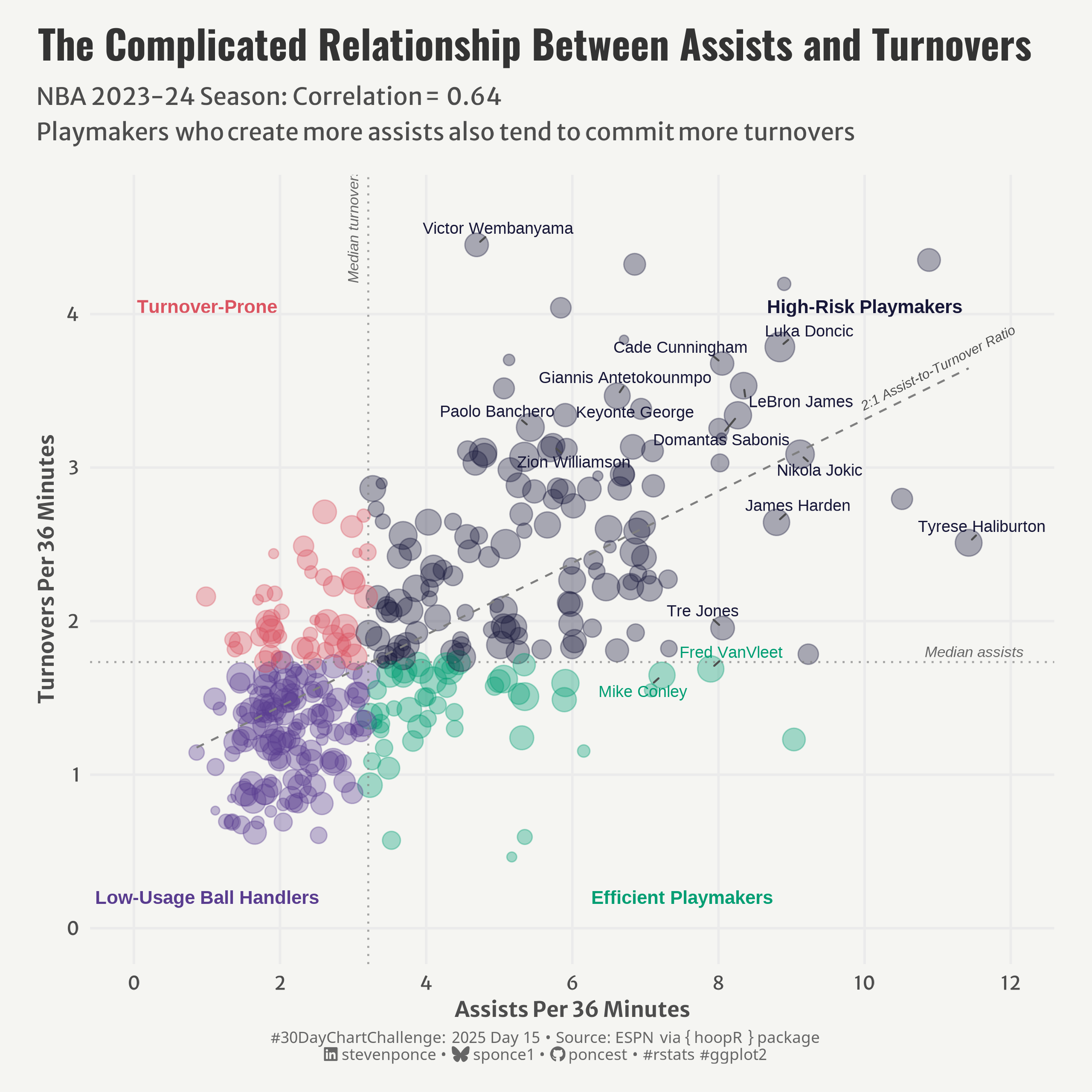See how elite playmakers like Haliburton and LeBron balance risk and reward." # twitter: true # linkedin: true # email: true # facebook: false # reddit: false # stumble: false # tumblr: false # mastodon: true # bsky: true --- ![Scatter plot showing NBA 2023-24 season data comparing assists versus turnovers per 36 minutes (correlation = 0.64). Players are divided into four categories: Efficient Playmakers, High-Risk Playmakers, Low-Usage Ball Handlers, and Turnover-Prone. Key players like Haliburton, Wembanyama, and James are labeled, illustrating the complicated relationship between playmaking and ball security.](30dcc_2025_15.png){#fig-1} ### <mark> **Steps to Create this Graphic** </mark> #### 1. Load Packages & Setup ```{r} #| label: load #| warning: false #| message: false #| results: "hide" ## 1. LOAD PACKAGES & SETUP ---- suppressPackageStartupMessages({ pacman::p_load( tidyverse, # Easily Install and Load the 'Tidyverse' ggtext, # Improved Text Rendering Support for 'ggplot2' showtext, # Using Fonts More Easily in R Graphs janitor, # Simple Tools for Examining and Cleaning Dirty Data skimr, # Compact and Flexible Summaries of Data scales, # Scale Functions for Visualization lubridate, # Make Dealing with Dates a Little Easier hoopR, # Access Men's Basketball Play by Play Data paletteer, # Comprehensive Collection of Color Palettes ggrepel, # Automatically Position Non-Overlapping Text Labels with ggplot2 camcorder # Record Your Plot History ) }) ### |- figure size ---- gg_record( dir = here::here("temp_plots"), device = "png", width = 8, height = 8, units = "in", dpi = 320 ) # Source utility functions suppressMessages(source(here::here("R/utils/fonts.R"))) source(here::here("R/utils/social_icons.R")) source(here::here("R/utils/image_utils.R")) source(here::here("R/themes/base_theme.R")) ``` #### 2. Read in the Data ```{r} #| label: read #| include: true #| eval: true #| warning: false # Get player stats for 2023-2024 season nba_players <- load_nba_player_box(seasons = 2024) ``` #### 3. Examine the Data ```{r} #| label: examine #| include: true #| eval: true #| results: 'hide' #| warning: false glimpse(nba_players) skim(nba_players) ``` #### 4. Tidy Data ```{r} #| label: tidy #| warning: false ### |- Tidy ---- # Calculate aggregate stats (assists and turnovers) player_stats <- nba_players |> group_by(athlete_display_name, athlete_position_name) |> summarize( games = n(), minutes = sum(minutes, na.rm = TRUE), assists = sum(assists, na.rm = TRUE), turnovers = sum(turnovers, na.rm = TRUE), ast_per_36 = (assists / minutes) * 36, tov_per_36 = (turnovers / minutes) * 36, ast_to_ratio = assists / pmax(turnovers, 0.5), .groups = "drop" ) |> filter( minutes >= 500, !is.na(ast_per_36), !is.na(tov_per_36), is.finite(ast_per_36), is.finite(tov_per_36) ) |> mutate( high_ast = ast_per_36 > median(ast_per_36), high_tov = tov_per_36 > median(tov_per_36), playmaker_type = case_when( high_ast & !high_tov ~ "Efficient Playmakers", high_ast & high_tov ~ "High-Risk Playmakers", !high_ast & !high_tov ~ "Low-Usage Ball Handlers", !high_ast & high_tov ~ "Turnover-Prone" ) ) # Correlation correlation <- cor( player_stats$ast_per_36, player_stats$tov_per_36, use = "complete.obs" ) # Label df elite_players <- player_stats |> filter( minutes > 1500 & ( # Elite point guards and playmakers ast_per_36 > quantile(player_stats$ast_per_36, 0.95) | # Players with unusual assist/turnover combos (ast_per_36 > 7 & tov_per_36 < 1.5) | tov_per_36 > quantile(player_stats$tov_per_36, 0.95) | # Super-efficient playmakers (ast_per_36 > 6 & ast_to_ratio > 4) | # manually selected a few stars athlete_display_name %in% c( "LeBron James", "Nikola Jokic", "Chris Paul", "Victor Wembanyama", "Tyrese Haliburton", "Joel Embiid" ) ) ) |> # Top N slice_max(order_by = minutes, n = 15) ``` #### 5. Visualization Parameters ```{r} #| label: params #| include: true #| warning: false ### |- plot aesthetics ---- colors <- get_theme_colors( palette = c( "Efficient Playmakers" = "#009E73", "High-Risk Playmakers" = "#171738", "Low-Usage Ball Handlers" = "#593C8F", "Turnover-Prone" = "#DB5461" ) ) ### |- titles and caption ---- # text title_text <- str_wrap("The Complicated Relationship Between Assists and Turnovers", width = 60) subtitle_text <- str_glue( "NBA 2023-24 Season: Correlation = { round(correlation, 2) }<br> Playmakers who create more assists also tend to commit more turnovers" ) caption_text <- create_dcc_caption( dcc_year = 2025, dcc_day = 15, source_text = "ESPN via { hoopR } package" ) ### |- fonts ---- setup_fonts() fonts <- get_font_families() ### |- plot theme ---- # Start with base theme base_theme <- create_base_theme(colors) # Add weekly-specific theme elements weekly_theme <- extend_weekly_theme( base_theme, theme( # Axis elements axis.title = element_text(color = colors$text, size = rel(0.8)), axis.text = element_text(color = colors$text, size = rel(0.7)), # Grid elements panel.grid.minor = element_blank(), panel.grid.major = element_line(color = "gray92"), # Legend elements legend.position = "plot", legend.title = element_text(family = fonts$text, size = rel(0.8)), legend.text = element_text(family = fonts$text, size = rel(0.7)), # Plot margins plot.margin = margin(t = 10, r = 20, b = 10, l = 20), ) ) # Set theme theme_set(weekly_theme) ``` #### 6. Plot ```{r} #| label: plot #| warning: false ### |- Plot ---- p <- ggplot(player_stats, aes(x = ast_per_36, y = tov_per_36, color = playmaker_type) ) + # Geoms geom_point( aes(size = minutes), alpha = 0.35 ) + geom_hline( yintercept = median(player_stats$tov_per_36), linetype = "dotted", color = "gray50", alpha = 0.7 ) + geom_vline( xintercept = median(player_stats$ast_per_36), linetype = "dotted", color = "gray50", alpha = 0.7 ) + geom_smooth( method = "lm", formula = y ~ x, se = FALSE, color = "gray50", linetype = "dashed", alpha = 0.5, linewidth = 0.5 ) + geom_text_repel( data = elite_players, aes(label = athlete_display_name), size = 3, max.overlaps = 10, box.padding = 0.3, point.padding = 0.2, segment.color = "gray30", min.segment.length = 0.2, force = 5, seed = 123 ) + # Scales scale_x_continuous( breaks = seq(0, 12, by = 2), limits = c(0, max(player_stats$ast_per_36) * 1.05) ) + scale_y_continuous( breaks = seq(0, 5, by = 1), limits = c(0, max(player_stats$tov_per_36) * 1.05) ) + scale_size_continuous( name = "Total Minutes Played", range = c(1.5, 7), breaks = c(1000, 2000, 3000) ) + scale_color_manual( values = colors$palette ) + # Labs labs( title = title_text, subtitle = subtitle_text, caption = caption_text, x = "Assists Per 36 Minutes", y = "Turnovers Per 36 Minutes", ) + # Annotate annotate( "text", x = 11.5, y = 1.8, label = "Median assists", fontface = "italic", size = 2.8, color = "gray40", hjust = 0.5 ) + annotate( "text", x = 3, y = 4.2, label = "Median turnovers", fontface = "italic", size = 2.8, color = "gray40", hjust = 0, angle = 90 ) + annotate( "text", x = 11, y = 3.65, label = "2:1 Assist-to-Turnover Ratio", fontface = "italic", size = 2.5, color = "gray30", angle = 27 ) + annotate( "text", x = 7.5, y = 0.2, label = "Efficient Playmakers", fontface = "bold", size = 3.5, color = colors$palette[1] ) + annotate( "text", x = 10, y = 4.05, label = "High-Risk Playmakers", fontface = "bold", size = 3.5, color = colors$palette[2] ) + annotate( "text", x = 1, y = 0.2, label = "Low-Usage Ball Handlers", fontface = "bold", size = 3.5, color = colors$palette[3] ) + annotate( "text", x = 1, y = 4.05, label = "Turnover-Prone", fontface = "bold", size = 3.5, color = colors$palette[4] ) + # Theme theme( plot.title = element_text( size = rel(1.5), family = fonts$title, face = "bold", color = colors$title, margin = margin(t = 5, b = 5) ), plot.subtitle = element_markdown( size = rel(0.9), family = fonts$subtitle, color = colors$subtitle, lineheight = 1.5, margin = margin(t = 5, b = 15) ), plot.caption = element_markdown( size = rel(0.6), family = fonts$caption, color = colors$caption, lineheight = 0.65, hjust = 0.5, halign = 0.5, margin = margin(t = 5, b = 5) ), ) ``` #### 7. Save ```{r} #| label: save #| warning: false ### |- plot image ---- save_plot( p, type = "30daychartchallenge", year = 2025, day = 15, width = 8, height = 8 ) ``` #### 8. Session Info ::: {.callout-tip collapse="true"} ##### Expand for Session Info ```{r, echo = FALSE} #| eval: true #| warning: false sessionInfo() ``` ::: #### 9. GitHub Repository ::: {.callout-tip collapse="true"} ##### Expand for GitHub Repo The complete code for this analysis is available in [`30dcc_2025_15.qmd`](https://github.com/poncest/personal-website/blob/master/data_visualizations/TidyTuesday/2025/30dcc_2025_15.qmd). For the full repository, [click here](https://github.com/poncest/personal-website/). ::: #### 10. References ::: {.callout-tip collapse="true"} ##### Expand for References 1. Data Sources: - ESPN via { hoopR } package: [hoopR](https://github.com/sportsdataverse/hoopR) :::