---
title: "Birds of a Feather: How NBA's Bird Teams Show Identical Home Nest Advantage"
subtitle: "Both Hawks and Pelicans win exactly 54.3% of home games and 45.7% of away games"
description: "Analyzing NBA's two bird-themed teams reveals a surprising statistical symmetry: both the Atlanta Hawks and New Orleans Pelicans share identical home and away win percentages during the 2023-24 season, demonstrating a perfect mirror image of home court advantage patterns."
date: "2025-04-17"
categories: ["30DayChartChallenge", "2025"]
tags: [
"ggplot2", "hoopR", "NBA", "Sports Analytics", "Home Court Advantage", "Atlanta Hawks", "New Orleans Pelicans", "Bird Teams", "Relationships", "Win Percentage"
]
image: "thumbnails/30dcc_2025_17.png"
format:
html:
toc: true
toc-depth: 5
code-link: true
code-fold: true
code-tools: true
code-summary: "Show code"
editor_options:
chunk_output_type: inline
execute:
freeze: true
cache: true
error: false
message: false
warning: false
eval: true
# filters:
# - social-share
# share:
# permalink: "https://stevenponce.netlify.app/data_visualizations/30DayChartChallenge/2025/30dcc_2025_17.html"
# description: "Day 17 of #30DayChartChallenge: Birds of a Feather - Discovering the identical home court advantage patterns shared by NBA's bird-themed teams"
# twitter: true
# linkedin: true
# email: true
# facebook: false
# reddit: false
# stumble: false
# tumblr: false
# mastodon: true
# bsky: true
---
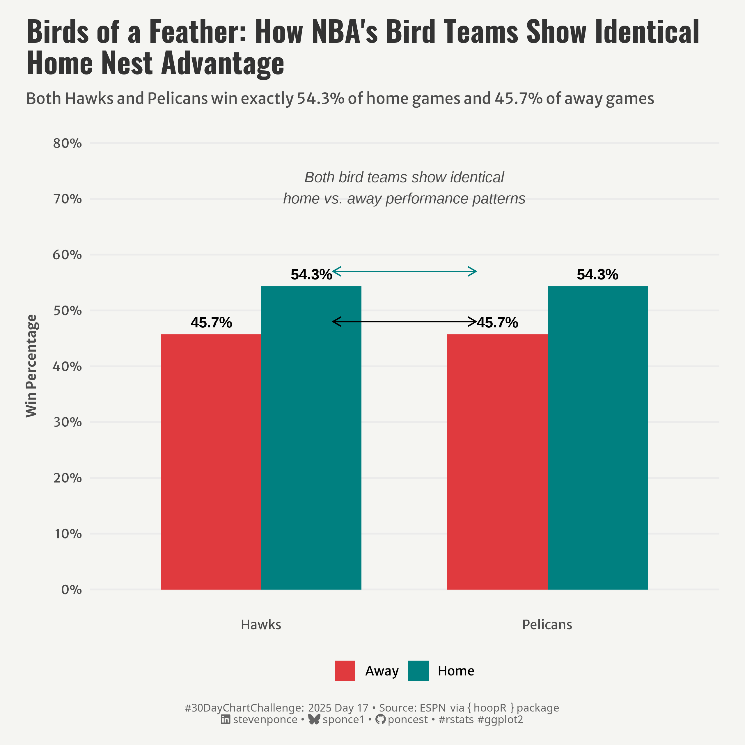{#fig-1}
### <mark> **Steps to Create this Graphic** </mark>
#### 1. Load Packages & Setup
```{r}
#| label: load
#| warning: false
#| message: false
#| results: "hide"
## 1. LOAD PACKAGES & SETUP ----
suppressPackageStartupMessages({
pacman::p_load(
  tidyverse,      # Easily Install and Load the 'Tidyverse'
  ggtext,         # Improved Text Rendering Support for 'ggplot2'
  showtext,       # Using Fonts More Easily in R Graphs
  janitor,        # Simple Tools for Examining and Cleaning Dirty Data
  skimr,          # Compact and Flexible Summaries of Data
  scales,         # Scale Functions for Visualization
  lubridate,      # Make Dealing with Dates a Little Easier
  hoopR,          # Access Men's Basketball Play by Play Data
  ggrepel,        # Automatically Position Non-Overlapping Text Labels with ggplot2
  camcorder       # Record Your Plot History
  )
})

### |- figure size ----
gg_record(
    dir    = here::here("temp_plots"),
    device = "png",
    width  = 8,
    height = 8,
    units  = "in",
    dpi    = 320
)

# Source utility functions
suppressMessages(source(here::here("R/utils/fonts.R")))
source(here::here("R/utils/social_icons.R"))
source(here::here("R/utils/image_utils.R"))
source(here::here("R/themes/base_theme.R"))
```
#### 2. Read in the Data
```{r}
#| label: read
#| include: true
#| eval: true
#| warning: false
# Define the bird teams using their NBA team IDs
pelicans_id <- "1610612740"  # New Orleans Pelicans
hawks_id <- "1610612737"     # Atlanta Hawks

# Get team game logs for the 2023-2024 season
pelicans_games <- hoopR::nba_leaguegamelog(season = "2023-24", team_id_nullable = pelicans_id)
hawks_games <- hoopR::nba_leaguegamelog(season = "2023-24", team_id_nullable = hawks_id)

# Extract and prepare data
pelicans_data <- pelicans_games$LeagueGameLog |> mutate(team = "Pelicans")
hawks_data <- hawks_games$LeagueGameLog |> mutate(team = "Hawks")

# Combine datasets
all_games <- bind_rows(pelicans_data, hawks_data)
```
#### 3. Examine the Data
```{r}
#| label: examine
#| include: true
#| eval: true
#| results: 'hide'
#| warning: false
glimpse(all_games)
skim(all_games)
```
#### 4. Tidy Data
```{r}
#| label: tidy
#| warning: false
### |- Tidy ----
# Add home/away indicator
all_games <- all_games |>
  mutate(location = if_else(MATCHUP |> str_detect("@"), "Away", "Home"))

# Calculate metrics
bird_analysis <- all_games |>
  mutate(
    game_date = as.Date(GAME_DATE, format = "%m/%d/%Y"),
    FGA_num = as.numeric(FGA),
    FTA_num = as.numeric(FTA),
    TOV_num = as.numeric(TOV),
    OREB_num = as.numeric(OREB),
    MIN_num = as.numeric(gsub(":", ".", MIN)),
    PTS_num = as.numeric(PTS),

    pace = case_when(
      is.na(MIN_num) | MIN_num == 0 ~ NA_real_,
      TRUE ~ (FGA_num + TOV_num + 0.44 * FTA_num - OREB_num) / MIN_num * 48
    ),

    efficiency = case_when(
      is.na(FGA_num) | FGA_num == 0 ~ NA_real_,
      TRUE ~ PTS_num / FGA_num
    )
  ) |>
  filter(!is.na(pace), !is.na(efficiency), !is.infinite(pace), !is.infinite(efficiency))

# Calculate home vs away statistics
home_away_summary <- bird_analysis |>
  group_by(team, location) |>
  summarize(
    avg_pace = mean(pace, na.rm = TRUE),
    avg_efficiency = mean(efficiency, na.rm = TRUE),
    games_played = n(),
    wins = sum(WL == "W", na.rm = TRUE),
    win_pct = wins / games_played,
    .groups = "drop"
  )
```
#### 5. Visualization Parameters
```{r}
#| label: params
#| include: true
#| warning: false
### |-  plot aesthetics ----
colors <- get_theme_colors(
  palette = c(
    "Home" = "#008080",
    "Away" = "#E03A3E"
  )
)

### |-  titles and caption ----
# text
title_text    <- str_wrap("Birds of a Feather: How NBA's Bird Teams Show Identical Home Nest Advantage",
                          width = 55)

subtitle_text <- str_wrap("Both Hawks and Pelicans win exactly 54.3% of home games and 45.7% of away games",
                          width = 85)

caption_text <- create_dcc_caption(
  dcc_year = 2025,
  dcc_day = 17,
  source_text =  "ESPN via { hoopR } package"
)

### |-  fonts ----
setup_fonts()
fonts <- get_font_families()

### |-  plot theme ----

# Start with base theme
base_theme <- create_base_theme(colors)

# Add weekly-specific theme elements
weekly_theme <- extend_weekly_theme(
  base_theme,
  theme(

    # Axis elements
    axis.title.y = element_text(color = colors$text, size = rel(0.8), margin = margin(r = 10)),
    axis.text = element_text(color = colors$text, size = rel(0.7)),

    # Grid elements
    panel.grid.minor = element_blank(),
    panel.grid.major.x = element_blank(),
    panel.grid.major.y = element_line(color = "gray92"),

    # Legend elements
    legend.position = "bottom",
    legend.title = element_blank(),
    # legend.title = element_text(family = fonts$text, size = rel(0.8)),
    legend.text = element_text(family = fonts$text, size = rel(0.7)),

    # Plot margins
    plot.margin = margin(t = 10, r = 20, b = 10, l = 20),
  )
)

# Set theme
theme_set(weekly_theme)
```
#### 6. Plot
```{r}
#| label: plot
#| warning: false
### |-  Plot ----
p <- ggplot(home_away_summary, aes(x = team, y = win_pct, fill = location)) +
  # Geoms
  geom_col(
    position = "dodge",
    width = 0.7
    ) +
  geom_text(
    aes(label = scales::percent(win_pct, accuracy = 0.1)),
    position = position_dodge(
      width = 0.7),
    vjust = -0.7,
    size = 4,
    fontface = "bold"
    ) +
  # Scales
  scale_y_continuous(
    labels = scales::percent, limits = c(0, 0.8),
    breaks = seq(0, 0.8, 0.1)
    ) +
  scale_fill_manual(
    values = colors$palette
    ) +
  # Annotate
  annotate(
    "text", x = 1.5, y = 0.72,
    label = "Both bird teams show identical\nhome vs. away performance patterns",
    size = 4, fontface = "italic", color = "gray30"
    ) +
  annotate(
    "segment", x = 1.25, xend = 1.75, y = 0.57, yend = 0.57,
    arrow = arrow(ends = "both", length = unit(0.1, "inches")),
    color = colors$palette[1]
    ) +
  annotate(
    "segment", x = 1.25, xend = 1.75, y = 0.48, yend = 0.48,
    arrow = arrow(ends = "both", length = unit(0.1, "inches")),
    olor = colors$palette[2]
    ) +
  # Labs
  labs(
    title = title_text,
    subtitle = subtitle_text,
    caption = caption_text,
    y = "Win Percentage",
    x = NULL,
  ) +
  # Theme
  theme(
    plot.title = element_text(
      size = rel(1.6),
      family = fonts$title,
      face = "bold",
      color = colors$title,
      margin = margin(t = 5, b = 5)
    ),
    plot.subtitle = element_text(
      size = rel(0.85),
      family = fonts$subtitle,
      color = colors$subtitle,
      lineheight = 1.2,
      margin = margin(t = 5, b = 10)
    ),
    plot.caption = element_markdown(
      size = rel(0.6),
      family = fonts$caption,
      color = colors$caption,
      lineheight = 0.65,
      hjust = 0.5,
      halign = 0.5,
      margin = margin(t = 10, b = 5)
    ),
  )
```
#### 7. Save
```{r}
#| label: save
#| warning: false
### |-  plot image ----

save_plot(
  p,
  type = "30daychartchallenge",
  year = 2025,
  day = 17,
  width = 8,
  height = 8
  )
```
#### 8. Session Info
::: {.callout-tip collapse="true"}
##### Expand for Session Info
```{r, echo = FALSE}
#| eval: true
#| warning: false
sessionInfo()
```
:::
#### 9. GitHub Repository
::: {.callout-tip collapse="true"}
##### Expand for GitHub Repo
The complete code for this analysis is available in [`30dcc_2025_17.qmd`](https://github.com/poncest/personal-website/blob/master/data_visualizations/TidyTuesday/2025/30dcc_2025_17.qmd).
For the full repository, [click here](https://github.com/poncest/personal-website/).
:::
#### 10. References
::: {.callout-tip collapse="true"}
##### Expand for References
1. Data Sources:
- ESPN via { hoopR } package: [hoopR](https://github.com/sportsdataverse/hoopR)
:::
