---
title: "Relationship Between Peak Hour and Daily Traffic"
subtitle: "Major corridors in Los Angeles and Orange counties show higher traffic volumes than Bay Area routes"
description: "Analysis of California traffic data showing the strong linear relationship between peak hour traffic volume and annual average daily traffic across different counties. This visualization, created for Day 18 of the #30DayChartChallenge with an El País-inspired design, reveals how traffic patterns vary between major urban areas."
date: "2025-04-18"
categories: ["30DayChartChallenge", "2025"]
tags: [
"ggplot2", "transportation", "urban planning", "El Pais", "traffic analysis", "California", "scatter plot", "relationships", "county comparison", "peak hour traffic"
]
image: "thumbnails/30dcc_2025_18.png"
format:
html:
toc: true
toc-depth: 5
code-link: true
code-fold: true
code-tools: true
code-summary: "Show code"
editor_options:
chunk_output_type: inline
execute:
freeze: true
cache: true
error: false
message: false
warning: false
eval: true
# filters:
# - social-share
# share:
# permalink: "https://stevenponce.netlify.app/data_visualizations/30DayChartChallenge/2025/30dcc_2025_18.html"
# description: "Day 18 of #30DayChartChallenge: Exploring the relationship between peak hour and daily traffic volumes across California counties in El País style"
# twitter: true
# linkedin: true
# email: true
# facebook: false
# reddit: false
# stumble: false
# tumblr: false
# mastodon: true
# bsky: true
---
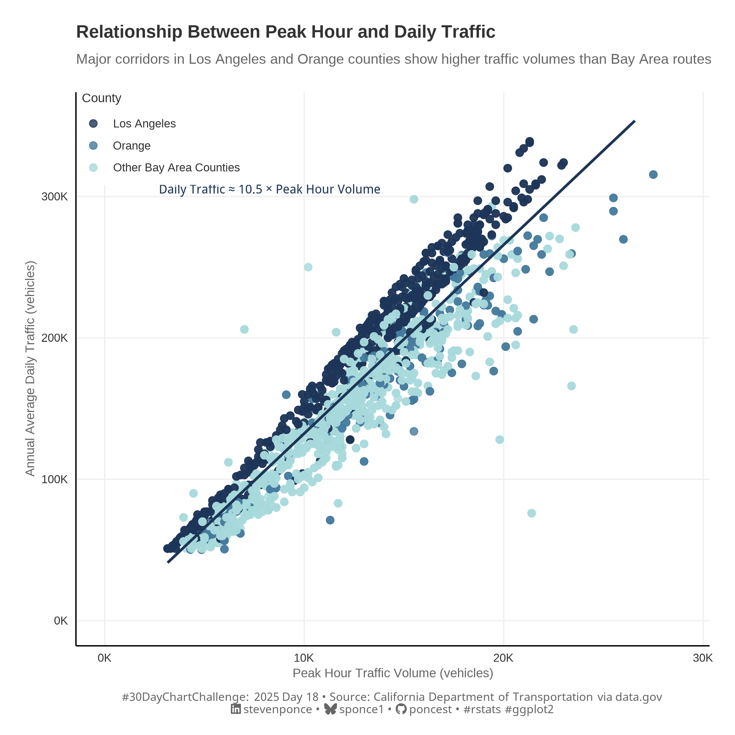{#fig-1}
### <mark> **Steps to Create this Graphic** </mark>
#### 1. Load Packages & Setup
```{r}
#| label: load
#| warning: false
#| message: false
#| results: "hide"
## 1. LOAD PACKAGES & SETUP ----
suppressPackageStartupMessages({
pacman::p_load(
  tidyverse,      # Easily Install and Load the 'Tidyverse'
  ggtext,         # Improved Text Rendering Support for 'ggplot2'
  showtext,       # Using Fonts More Easily in R Graphs
  janitor,        # Simple Tools for Examining and Cleaning Dirty Data
  skimr,          # Compact and Flexible Summaries of Data
  scales,         # Scale Functions for Visualization
  lubridate,      # Make Dealing with Dates a Little Easier
  camcorder       # Record Your Plot History
  )
})

### |- figure size ----
gg_record(
    dir    = here::here("temp_plots"),
    device = "png",
    width  = 8,
    height = 8,
    units  = "in",
    dpi    = 320
)

# Source utility functions
suppressMessages(source(here::here("R/utils/fonts.R")))
source(here::here("R/utils/social_icons.R"))
source(here::here("R/utils/image_utils.R"))
source(here::here("R/themes/base_theme.R"))
```
#### 2. Read in the Data
```{r}
#| label: read
#| include: true
#| eval: true
#| warning: false
traffic_volumnes_raw <- read_csv(here::here(
  'data/30DayChartChallenge/2025/Traffic_Volumes_AADT.csv')
  ) |>
    clean_names()
```
#### 3. Examine the Data
```{r}
#| label: examine
#| include: true
#| eval: true
#| results: 'hide'
#| warning: false
glimpse(traffic_volumnes_raw)
skim(traffic_volumnes_raw)
```
#### 4. Tidy Data
```{r}
#| label: tidy
#| warning: false
### |- Tidy ----
simple_traffic <- traffic_volumnes_raw |>
  select(county, route, back_peak_hour, back_aadt) |>
  filter(!is.na(back_peak_hour) & !is.na(back_aadt)) |>
  # Major counties with substantial data
  filter(county %in% c("LA", "SD", "ORA", "SF", "SCL", "ALA", "CC")) |>
  # Routes with higher traffic
  filter(back_aadt > 50000) |>
  # Remove extreme outliers (values beyond 3x the standard deviation)
  filter(
    back_peak_hour < mean(back_peak_hour) + 3*sd(back_peak_hour),
    back_aadt < mean(back_aadt) + 3*sd(back_aadt)
  ) |>
  mutate(
    peak_ratio = back_peak_hour / (back_aadt/24),
    county_group = case_when(
      county == "LA" ~ "Los Angeles",
      county == "ORA" ~ "Orange",
      TRUE ~ "Other Bay Area Counties"
    )
  )
```
#### 5. Visualization Parameters
```{r}
#| label: params
#| include: true
#| warning: false
### |-  plot aesthetics ----
colors <- get_theme_colors(
  palette = c(
    "Los Angeles" = "#1D3557",
    "Orange" = "#457B9D",
    "Other Bay Area Counties" = "#A8DADC" ,
    NULL = "#A8DADC40"
  )
)

### |-  titles and caption ----
# text
title_text    <- str_glue("Relationship Between Peak Hour and Daily Traffic")

subtitle_text <- str_glue("Major corridors in Los Angeles and Orange counties show higher traffic volumes than Bay Area routes")

caption_text <- create_dcc_caption(
  dcc_year = 2025,
  dcc_day = 18,
  source_text =  "California Department of Transportation via data.gov"
)

### |-  fonts ----
setup_fonts()
fonts <- get_font_families()

### |-  plot theme ----

# El País theme (at least my interpretation)
el_pais_theme <- function() {
  theme_minimal(base_size = 14) +
    theme(
      # Typography
      text = element_text(family = "Helvetica", color = "#333333"),
      plot.title = element_text(size = rel(1), face = "bold", hjust = 0, margin = margin(b = 10)),
      plot.subtitle = element_text(size = rel(0.79), color = "#666666", hjust = 0, margin = margin(b = 20)),

      # Axis styling
      axis.title = element_text(size = rel(0.71), color = "#666666"),
      axis.text = element_text(size = rel(0.64), color = "#333333"),
      axis.line = element_line(color = "black", linewidth = 0.5),

      # Grid styling
      panel.grid.major = element_line(color = "#f0f0f0", linewidth = 0.5),
      panel.grid.minor = element_blank(),

      # Legend styling
      legend.title = element_text(size = rel(0.71)),
      legend.text = element_text(size = rel(0.64)),
      legend.position = c(0.01, 1),
      legend.justification = c(0, 1),
      legend.background = element_rect(fill = "white", color = NA),
      legend.key.size = unit(1.2, "lines"),
      legend.margin = margin(t = 0, r = 10, b = 5, l = 0),

      # Margins & Others
      plot.margin = margin(t = 20, r = 20, b = 15, l = 20),
      plot.background = element_rect(fill = 'white', color = 'white'),
      panel.background = element_rect(fill = 'white', color = 'white')
    )
}
```
#### 6. Plot
```{r}
#| label: plot
#| warning: false
### |-  Plot ----
p <- ggplot(simple_traffic, aes(x = back_peak_hour, y = back_aadt)) +
  # Geoms
  geom_point(
    aes(color = county_group),
    alpha = 0.8,
    size = 2.5
  ) +
  geom_smooth(
    method = "lm",
    formula = y ~ x,
    color = colors$palette[1],
    fill = colors$palette[5],
    size = 1,
    fullrange = FALSE  # Only draw the trend line within the range of actual data
  ) +
  # Annotate
  annotate(
    "text",
    x = max(simple_traffic$back_peak_hour) * 0.3,
    y = max(simple_traffic$back_aadt) * 0.9,
    label = "Daily Traffic ≈ 10.5 × Peak Hour Volume",
    color = colors$palette[1],
    fontface = "italic",
    size = 3.5
  ) +
  # Scales
  scale_color_manual(
    values = colors$palette,
    name = "County"
  ) +
  scale_y_continuous(
    labels = function(x) paste0(x/1000, "K"),
    name = "Annual Average Daily Traffic (vehicles)",
    limits = c(0, max(simple_traffic$back_aadt) * 1.05)
  ) +
  scale_x_continuous(
    labels = function(x) paste0(x/1000, "K"),
    name = "Peak Hour Traffic Volume (vehicles)",
    limits = c(0, max(simple_traffic$back_peak_hour) * 1.05)
  ) +
  # Labs
  labs(
    title = title_text,
    subtitle = subtitle_text,
    caption = caption_text
  ) +
  # Theme
  el_pais_theme() +
  theme(
    plot.caption = element_markdown(
      size = rel(0.65),
      family = fonts$caption,
      color = colors$caption,
      hjust = 0.5,
      margin = margin(t = 10)
    )
  )
```
#### 7. Save
```{r}
#| label: save
#| warning: false
### |-  plot image ----

save_plot(
  p,
  type = "30daychartchallenge",
  year = 2025,
  day = 18,
  width = 8,
  height = 8
  )
```
#### 8. Session Info
::: {.callout-tip collapse="true"}
##### Expand for Session Info
```{r, echo = FALSE}
#| eval: true
#| warning: false
sessionInfo()
```
:::
#### 9. GitHub Repository
::: {.callout-tip collapse="true"}
##### Expand for GitHub Repo
The complete code for this analysis is available in [`30dcc_2025_18.qmd`](https://github.com/poncest/personal-website/blob/master/data_visualizations/TidyTuesday/2025/30dcc_2025_18.qmd).
For the full repository, [click here](https://github.com/poncest/personal-website/).
:::
#### 10. References
::: {.callout-tip collapse="true"}
##### Expand for References
1. Data Sources:
- California Annual Average Daily Traffic Volumes, Metadata Updated: November 27, 2024 [data.gov](https://catalog.data.gov/dataset/traffic-volumes-aadt-ee8d6)
:::
