---
title: "Rise and Fall of Trilobites: Fossil Records Over Time"
subtitle: "Exploring the dramatic rise and fall of one of Earth's most successful early arthropod groups"
description: "Visualizing 250 million years of trilobite fossil records from the Paleobiology Database, showing how these ancient arthropods dominated the Ordovician seas before declining after major extinction events."
date: "2025-04-21"
categories: ["30DayChartChallenge", "2025"]
tags: [
"paleontology", "trilobites", "extinction events", "paleobioDB", "fossil records", "timeseries", "ggplot2", "evolutionary history", "Ordovician", "Silurian", "Devonian"
]
image: "thumbnails/30dcc_2025_21.png"
format:
html:
toc: true
toc-depth: 5
code-link: true
code-fold: true
code-tools: true
code-summary: "Show code"
editor_options:
chunk_output_type: inline
execute:
freeze: true
cache: true
error: false
message: false
warning: false
eval: true
# filters:
# - social-share
# share:
# permalink: "https://stevenponce.netlify.app/data_visualizations/30DayChartChallenge/2025/30dcc_2025_21.html"
# description: "Day 21 of #30DayChartChallenge: Exploring trilobite fossil records over 250 million years, revealing their rise during the Ordovician and decline following major extinction events."
# twitter: true
# linkedin: true
# email: true
# facebook: false
# reddit: false
# stumble: false
# tumblr: false
# mastodon: true
# bsky: true
---
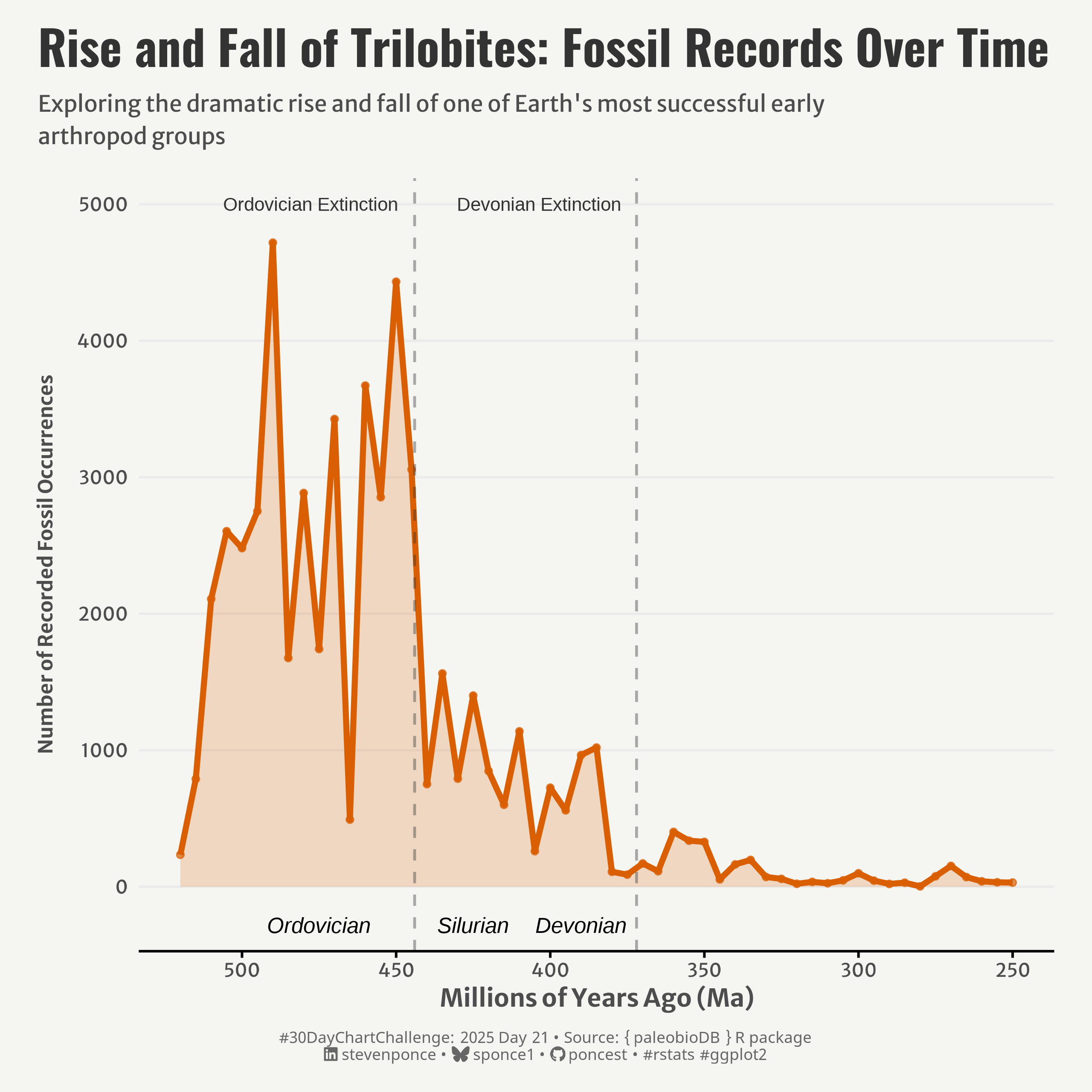{#fig-1}
### <mark> **Steps to Create this Graphic** </mark>
#### 1. Load Packages & Setup
```{r}
#| label: load
#| warning: false
#| message: false
#| results: "hide"
## 1. LOAD PACKAGES & SETUP ----
suppressPackageStartupMessages({
pacman::p_load(
  tidyverse,      # Easily Install and Load the 'Tidyverse'
  ggtext,         # Improved Text Rendering Support for 'ggplot2'
  showtext,       # Using Fonts More Easily in R Graphs
  janitor,        # Simple Tools for Examining and Cleaning Dirty Data
  skimr,          # Compact and Flexible Summaries of Data
  scales,         # Scale Functions for Visualization
  lubridate,      # Make Dealing with Dates a Little Easier
  paleobioDB,     # Download and Process Data from the Paleobiology Database # Download and Process Data from the Paleobiology Database
  ggrepel,        # Automatically Position Non-Overlapping Text Labels with 'ggplot2'
  camcorder       # Record Your Plot History
  )
})

### |- figure size ----
gg_record(
    dir    = here::here("temp_plots"),
    device = "png",
    width  = 8,
    height = 8,
    units  = "in",
    dpi    = 320
)

# Source utility functions
suppressMessages(source(here::here("R/utils/fonts.R")))
source(here::here("R/utils/social_icons.R"))
source(here::here("R/utils/image_utils.R"))
source(here::here("R/themes/base_theme.R"))
```
#### 2. Read in the Data
```{r}
#| label: read
#| include: true
#| eval: true
#| warning: false
# Search for fossil occurrences of trilobites
trilobites <- pbdb_occurrences(
  base_name = "Trilobita",
  show = c("time", "coords", "phylo"),
  limit = "all"
  )
```
#### 3. Examine the Data
```{r}
#| label: examine
#| include: true
#| eval: true
#| results: 'hide'
#| warning: false
glimpse(trilobites)
skim(trilobites)
```
#### 4. Tidy Data
```{r}
#| label: tidy
#| warning: false
### |- Tidy ----
trilo_time_binned <- trilobites |>
  filter(!is.na(eag), !is.na(lag)) |>
  mutate(
    mid_ma = (eag + lag) / 2,
    bin_5ma = floor(mid_ma / 5) * 5 ,
    bin_10ma = floor(mid_ma / 10) * 10
  ) |>
  count(bin_5ma) |>
  arrange(desc(bin_5ma))
```
#### 5. Visualization Parameters
```{r}
#| label: params
#| include: true
#| warning: false
### |-  plot aesthetics ----
colors <- get_theme_colors(
  palette = c(
    "#D95F02" ,
    "gray20"
  )
)

### |-  titles and caption ----
# text
title_text    <- str_wrap("Rise and Fall of Trilobites: Fossil Records Over Time",
                          width = 55)

subtitle_text <- str_wrap("Exploring the dramatic rise and fall of one of Earth's most successful early arthropod groups",
                          width = 85)

caption_text <- create_dcc_caption(
  dcc_year = 2025,
  dcc_day = 21,
  source_text =  "{ paleobioDB } R package"
)

### |-  fonts ----
setup_fonts()
fonts <- get_font_families()

### |-  plot theme ----

# Start with base theme
base_theme <- create_base_theme(colors)

# Add weekly-specific theme elements
weekly_theme <- extend_weekly_theme(
  base_theme,
  theme(

    # Axis elements
    axis.title.y = element_text(color = colors$text, size = rel(0.8), margin = margin(r = 10)),
    axis.text = element_text(color = colors$text, size = rel(0.7)),
    axis.line.x = element_line(color = "black"),
    axis.ticks.x = element_line(color = "black"),

    # Grid elements
    panel.grid.minor = element_blank(),
    panel.grid.major.x = element_blank(),
    panel.grid.major.y = element_line(color = "gray92"),

    # Legend elements
    legend.position = "plot",
    legend.title = element_blank(),
    legend.text = element_text(family = fonts$text, size = rel(0.7)),

    # Facet elements
    strip.background = element_rect(fill = "gray90", color = NA),
    strip.text = element_text(face = "bold", size = rel(1), margin = margin(10, 0, 10, 0)),

    # Plot margins
    plot.margin = margin(t = 10, r = 20, b = 10, l = 20),
  )
)

# Set theme
theme_set(weekly_theme)
```
#### 6. Plot
```{r}
#| label: plot
#| warning: false
### |-  Plot ----
p <- ggplot(trilo_time_binned, aes(x = bin_5ma, y = n)) +
  # Geoms
  geom_area(fill = colors$palette[1], alpha = 0.2) +
  geom_line(color = colors$palette[1], linewidth = 1.5) +
  geom_point(color = colors$palette[1], size = 1.5, alpha = 0.7) +
  geom_vline(xintercept = 444, linetype = "dashed", color = colors$palette[2], alpha = 0.4, linewidth = 0.7) +
  geom_vline(xintercept = 372, linetype = "dashed", color = colors$palette[2], alpha = 0.4, linewidth = 0.7) +
  # Annotate
  annotate("text",
    x = 444, y = 5000,
    label = "Ordovician Extinction",
    color = colors$palette[2], hjust = 1.1, size = 3.5
  ) +
  annotate("text",
    x = 372, y = 5000,
    label = "Devonian Extinction",
    color = colors$palette[2], hjust = 1.1, size = 3.5
  ) +
  annotate("text",
    x = 475, y = -283.8,
    label = "Ordovician", fontface = "italic", size = 4
  ) +
  annotate("text",
    x = 425, y = -283.8,
    label = "Silurian", fontface = "italic", size = 4
  ) +
  annotate("text",
    x = 390, y = -283.8,
    label = "Devonian", fontface = "italic", size = 4
  ) +
  # Scales
  scale_x_reverse(
    limits = c(520, 250),
    breaks = seq(500, 250, by = -50),
    minor_breaks = seq(500, 250, by = -10)
  ) +
  scale_y_continuous(
    limits = c(-max(trilo_time_binned$n) * 0.1, max(trilo_time_binned$n) * 1.1),
    expand = c(0, 0)
  ) +
  # Labs
  labs(
    title = title_text,
    subtitle = subtitle_text,
    caption = caption_text,
    x = "Millions of Years Ago (Ma)",
    y = "Number of Recorded Fossil Occurrences",
  ) +
  # Theme
  theme(
    plot.title = element_text(
      size = rel(1.8),
      family = fonts$title,
      face = "bold",
      color = colors$title,
      margin = margin(t = 5, b = 5)
    ),
    plot.subtitle = element_text(
      size = rel(0.85),
      family = fonts$subtitle,
      color = colors$subtitle,
      lineheight = 1.2,
      margin = margin(t = 5, b = 15)
    ),
    plot.caption = element_markdown(
      size = rel(0.6),
      family = fonts$caption,
      color = colors$caption,
      lineheight = 0.65,
      hjust = 0.5,
      halign = 0.5,
      margin = margin(t = 10, b = 5)
    ),
  )
```
#### 7. Save
```{r}
#| label: save
#| warning: false
### |-  plot image ----

save_plot(
  p,
  type = "30daychartchallenge",
  year = 2025,
  day = 21,
  width = 8,
  height = 8
  )
```
#### 8. Session Info
::: {.callout-tip collapse="true"}
##### Expand for Session Info
```{r, echo = FALSE}
#| eval: true
#| warning: false
sessionInfo()
```
:::
#### 9. GitHub Repository
::: {.callout-tip collapse="true"}
##### Expand for GitHub Repo
The complete code for this analysis is available in [`30dcc_2025_21.qmd`](https://github.com/poncest/personal-website/blob/master/data_visualizations/TidyTuesday/2025/30dcc_2025_21.qmd).
For the full repository, [click here](https://github.com/poncest/personal-website/).
:::
#### 10. References
::: {.callout-tip collapse="true"}
##### Expand for References
1. Data Sources:
- Paleobiology Database { paleobioDB } [indicator = Trilobita)](https://github.com/ropensci/paleobioDB)
:::
