---
title: "NBA Team Risk Matrix (2023-24 Season)"
subtitle: "Mapping team performance uncertainty against win probability"
description: "This NBA risk matrix visualizes team performance uncertainty against win probability for the 2023-24 season. By mapping standard deviation of point differential against win percentage, it reveals which teams are consistently good performers versus those with unpredictable outcomes. The visualization highlights risk quadrants and uses color to indicate average point differential, with circle size representing the likelihood of blowout losses."
date: "2025-04-25"
categories: ["30DayChartChallenge", "2025"]
tags: [
"ggplot2", "NBA", "sports analytics", "uncertainty visualization", "risk assessment", "basketball", "performance metrics", "statistical analysis", "hoopR", "point differential", "variance analysis", "win probability", "quadrant chart", "risk matrix"
]
image: "thumbnails/30dcc_2025_25.png"
format:
html:
toc: true
toc-depth: 5
code-link: true
code-fold: true
code-tools: true
code-summary: "Show code"
editor_options:
chunk_output_type: inline
execute:
freeze: true
cache: true
error: false
message: false
warning: false
eval: true
# filters:
# - social-share
# share:
# permalink: "https://stevenponce.netlify.app/data_visualizations/30DayChartChallenge/2025/30dcc_2025_25.html"
# description: "Day 25 of #30DayChartChallenge: Uncertainties and Risk - An NBA team risk matrix showing performance variability and win probability. Which teams are consistently good and which are unpredictably risky?"
# twitter: true
# linkedin: true
# email: true
# facebook: false
# reddit: false
# stumble: false
# tumblr: false
# mastodon: true
# bsky: true
---
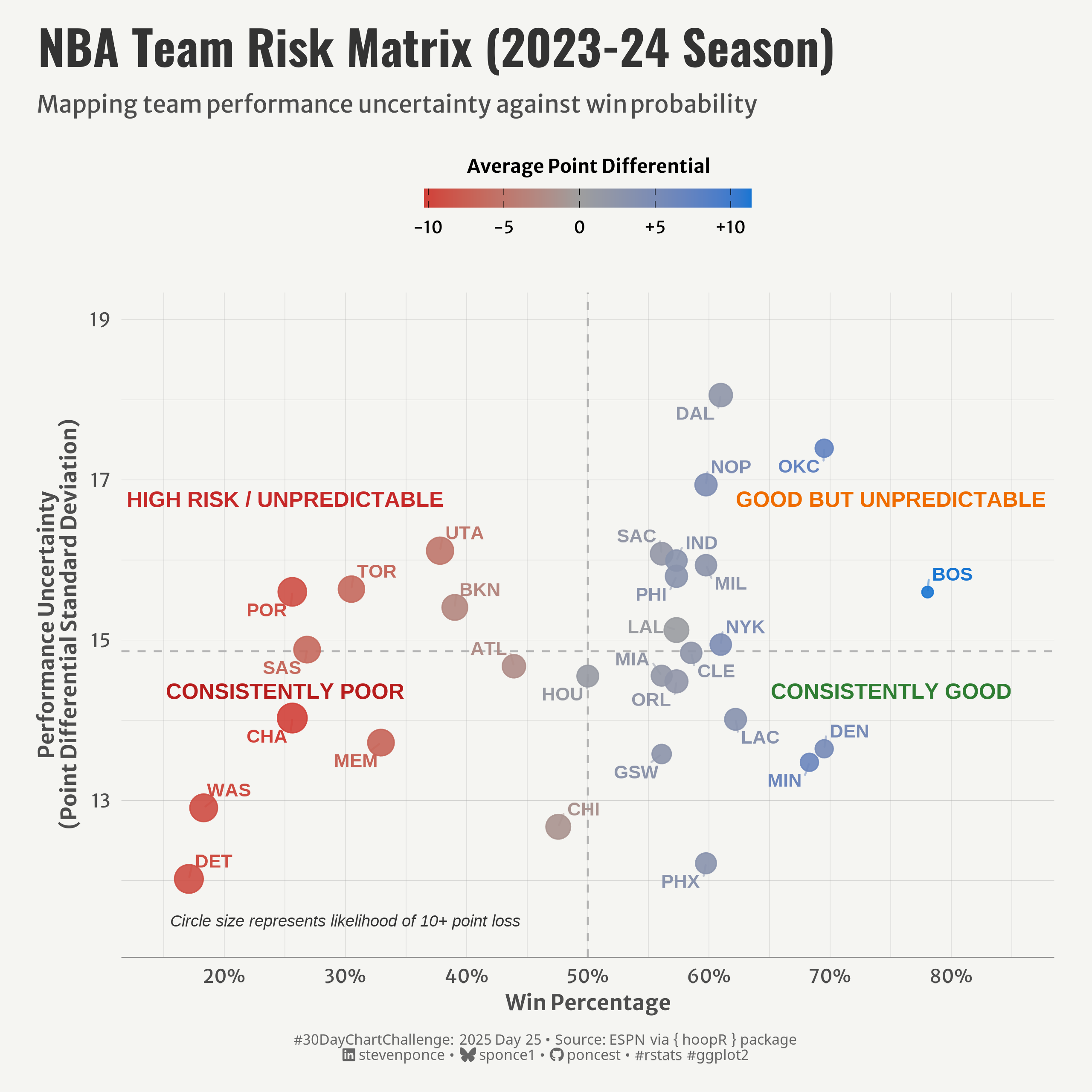{#fig-1}
### <mark> **Steps to Create this Graphic** </mark>
#### 1. Load Packages & Setup
```{r}
#| label: load
#| warning: false
#| message: false
#| results: "hide"
## 1. LOAD PACKAGES & SETUP ----
suppressPackageStartupMessages({
pacman::p_load(
   tidyverse,      # Easily Install and Load the 'Tidyverse'
  ggtext,         # Improved Text Rendering Support for 'ggplot2'
  showtext,       # Using Fonts More Easily in R Graphs
  janitor,        # Simple Tools for Examining and Cleaning Dirty Data
  skimr,          # Compact and Flexible Summaries of Data
  scales,         # Scale Functions for Visualization
  lubridate,      # Make Dealing with Dates a Little Easier
  ggrepel,        # Automatically Position Non-Overlapping Text Labels with 'ggplot2'
  hoopR,          # Access Men's Basketball Play by Play Data'
  camcorder       # Record Your Plot History
  )
})

### |- figure size ----
gg_record(
    dir    = here::here("temp_plots"),
    device = "png",
    width  = 8,
    height = 8,
    units  = "in",
    dpi    = 320
)

# Source utility functions
suppressMessages(source(here::here("R/utils/fonts.R")))
source(here::here("R/utils/social_icons.R"))
source(here::here("R/utils/image_utils.R"))
source(here::here("R/themes/base_theme.R"))
```
#### 2. Read in the Data
```{r}
#| label: read
#| include: true
#| eval: true
#| warning: false
# Get game results data for the 2023-24 season
games <- nba_leaguegamefinder(season = "2023-24")
games_data <- games$LeagueGameFinderResults
```
#### 3. Examine the Data
```{r}
#| label: examine
#| include: true
#| eval: true
#| results: 'hide'
#| warning: false
glimpse(games_data)
skim(games_data)
```
#### 4. Tidy Data
```{r}
#| label: tidy
#| warning: false
### |- Tidy ----
games_data <- games_data |>
  mutate(
    PLUS_MINUS = as.numeric(PLUS_MINUS),
    GAME_DATE = as.Date(GAME_DATE),
    PTS = as.numeric(PTS),
    OPP_PTS = as.numeric(PTS) - as.numeric(PLUS_MINUS)
  )

team_variability <- games_data |>
  group_by(TEAM_NAME) |>
  summarize(
    games_played = n(),
    avg_points = mean(as.numeric(PTS)),
    avg_point_diff = mean(PLUS_MINUS),
    points_sd = sd(as.numeric(PTS)),
    margin_sd = sd(PLUS_MINUS),
    win_pct = sum(WL == "W") / n(),
    blowout_risk = sum(PLUS_MINUS <= -10) / games_played,
    team_abbr = first(TEAM_ABBREVIATION),
    .groups = "drop"
  ) |>
  filter(games_played >= 10) |>
  arrange(desc(margin_sd))
```
#### 5. Visualization Parameters
```{r}
#| label: params
#| include: true
#| warning: false
### |-  plot aesthetics ----
colors <- get_theme_colors(
  palette = c(
    "#C62828", "#EF6C00", "#B71C1C", "#2E7D32",
    "#D32F2F", "#9E9E9E", "#1976D2"
    )
  )

### |-  titles and caption ----
# text
title_text    <- str_wrap("NBA Team Risk Matrix (2023-24 Season)",
                          width = 60)

subtitle_text <- str_wrap("Mapping team performance uncertainty against win probability",
                          width = 60)

caption_text <- create_dcc_caption(
  dcc_year = 2025,
  dcc_day = 25,
  source_text =  "ESPN via { hoopR } package"
)

### |-  fonts ----
setup_fonts()
fonts <- get_font_families()

### |-  plot theme ----

# Start with base theme
base_theme <- create_base_theme(colors)

# Add weekly-specific theme elements
weekly_theme <- extend_weekly_theme(
  base_theme,
  theme(

    # Text styling
    plot.title = element_text(face = "bold", family = fonts$title, size = rel(1.14), margin = margin(b = 10)),
    plot.subtitle = element_text(family = fonts$subtitle, color = colors$text, size = rel(0.78), margin = margin(b = 20)),

    # Axis elements
    axis.title = element_text(color = colors$text, size = rel(0.8)),
    axis.text = element_text(color = colors$text, size = rel(0.7)),

    axis.line.x = element_line(color = "gray50", linewidth = .2),

    # Grid elements
    panel.grid.minor = element_line(color = "gray65", linewidth = 0.05),
    panel.grid.major = element_line(color = "gray65", linewidth = 0.05),

    # Legend elements
    legend.position = "top",
    legend.margin = margin(t = 5, b = 15),
    legend.background = element_rect(fill = NA, color = NA),
    legend.key = element_rect(fill = NA, color = NA),
    legend.title = element_text(size = rel(0.71), face = "bold"),
    legend.text = element_text(size = rel(0.64)),

    # Plot margins
    plot.margin = margin(t = 10, r = 20, b = 10, l = 20),
  )
)

# Set theme
theme_set(weekly_theme)
```
#### 6. Plot
```{r}
#| label: plot
#| warning: false
### |-  Plot ----
p <- ggplot(team_variability,
       aes(x = win_pct, y = margin_sd)) +
  # Geoms
  geom_hline(
    yintercept = median(team_variability$margin_sd),
    linetype = "dashed", color = "gray70", size = 0.5
    ) +
  geom_vline(
    xintercept = 0.5, linetype = "dashed",
    color = "gray70", size = 0.5
    ) +
  geom_point(
    aes(size = blowout_risk, color = avg_point_diff),
    alpha = 0.9, stroke = 0.5
    ) +
  geom_text_repel(
    aes(label = team_abbr, color = avg_point_diff),
    size = 3.5, fontface = "bold", box.padding = 0.35,
    min.segment.length = 0.2, segment.alpha = 0.5,
    force = 1, max.overlaps = 15, seed = 123
    ) +
  # Annotate
  annotate(
    "text", x = 0.25, y = max(team_variability$margin_sd) - 1.3,
    label = "HIGH RISK / UNPREDICTABLE", color = colors$palette[1], fontface = "bold", size = 4
    ) +
  annotate(
    "text", x = 0.75, y = max(team_variability$margin_sd) - 1.3,
    label = "GOOD BUT UNPREDICTABLE", color = colors$palette[2], fontface = "bold", size = 4
    ) +
  annotate(
    "text", x = 0.25, y = median(team_variability$margin_sd) - 0.5,
    label = "CONSISTENTLY POOR", color = colors$palette[3], fontface = "bold", size = 4
    ) +
  annotate(
    "text", x = 0.75, y = median(team_variability$margin_sd) - 0.5,
    label = "CONSISTENTLY GOOD", color = colors$palette[4], fontface = "bold", size = 4
    ) +
  annotate(
    "text", x = 0.3, y = 11.5,
    label = "Circle size represents likelihood of 10+ point loss",
    color = "#333333", size = 3, fontface = "italic"
    ) +
  # Scales
  scale_color_gradient2(
    low = colors$palette[5], mid = colors$palette[6], high = colors$palette[7],
    midpoint = 0,
    name = "Average Point Differential",
    breaks = c(-10, -5, 0, 5, 10),
    labels = c("-10", "-5", "0", "+5", "+10"),
    guide = guide_colorbar(
      title.position = "top",
      title.hjust = 0.5,
      barwidth = 12,
      barheight = 0.7,
      frame.colour = NA,
      ticks.colour = "black"
    )
  ) +
  scale_size_continuous(
    range = c(2.5, 7),
    guide = "none"
  ) +
  scale_x_continuous(
    labels = percent_format(accuracy = 1),
    limits = c(0.15, 0.85),
    breaks = seq(0.2, 0.8, by = 0.1)
  ) +
  scale_y_continuous(
    limits = c(min(team_variability$margin_sd) * 0.95, max(team_variability$margin_sd) * 1.05)
  ) +
  # Labs
  labs(
    title = title_text,
    subtitle = subtitle_text,
    caption = caption_text,
    x = "Win Percentage",
    y = "Performance Uncertainty\n(Point Differential Standard Deviation)",
  ) +
  # Theme
  theme(
    plot.title = element_text(
      size = rel(1.8),
      family = fonts$title,
      face = "bold",
      color = colors$title,
      margin = margin(t = 5, b = 5)
    ),
    plot.subtitle = element_markdown(
      size = rel(0.9),
      family = fonts$subtitle,
      color = colors$subtitle,
      lineheight = 1.1,
      margin = margin(t = 5, b = 15)
    ),
    plot.caption = element_markdown(
      size = rel(0.55),
      family = fonts$caption,
      color = colors$caption,
      lineheight = 0.65,
      hjust = 0.5,
      halign = 0.5,
      margin = margin(t = 10, b = 5)
    ),
  )
```
#### 7. Save
```{r}
#| label: save
#| warning: false
### |-  plot image ----
save_plot(
  p,
  type = "30daychartchallenge",
  year = 2025,
  day = 25,
  width = 8,
  height = 8
  )
```
#### 8. Session Info
::: {.callout-tip collapse="true"}
##### Expand for Session Info
```{r, echo = FALSE}
#| eval: true
#| warning: false
sessionInfo()
```
:::
#### 9. GitHub Repository
::: {.callout-tip collapse="true"}
##### Expand for GitHub Repo
The complete code for this analysis is available in [`30dcc_2025_25.qmd`](https://github.com/poncest/personal-website/blob/master/data_visualizations/TidyTuesday/2025/30dcc_2025_25.qmd).
For the full repository, [click here](https://github.com/poncest/personal-website/).
:::
#### 10. References
::: {.callout-tip collapse="true"}
##### Expand for References
1. Data Sources:
- ESPN via { hoopR } package: [hoopR](https://github.com/sportsdataverse/hoopR)
:::
