---
title: "Uncertainty in Cardiovascular Disease Prevalence Across the U.S."
subtitle: "95% confidence intervals for states and territories reveal varying levels of statistical precision (CDC, 2023)"
description: "A visualization of cardiovascular disease prevalence across U.S. states and territories, highlighting statistical uncertainty through confidence intervals. This chart demonstrates how sample sizes affect the precision of health statistics, with wider intervals indicating less certainty in the estimate."
date: "2025-04-26"
categories: ["30DayChartChallenge", "2025"]
tags: [
"uncertainty",
"public health",
"confidence intervals",
"cardiovascular disease",
"CDC",
"BRFSS",
"statistical precision",
"monochrome",
"ggplot2",
"epidemiology"
]
image: "thumbnails/30dcc_2025_26.png"
format:
html:
toc: true
toc-depth: 5
code-link: true
code-fold: true
code-tools: true
code-summary: "Show code"
editor_options:
chunk_output_type: inline
execute:
freeze: true
cache: true
error: false
message: false
warning: false
eval: true
# filters:
# - social-share
# share:
# permalink: "https://stevenponce.netlify.app/data_visualizations/30DayChartChallenge/2025/30dcc_2025_26.html"
# description: "Day 26 of #30DayChartChallenge: Uncertainty in Cardiovascular Disease Prevalence. This visualization shows how confidence intervals reveal varying levels of statistical precision in public health data across U.S. states and territories. #dataviz #rstats #publichealth"
# twitter: true
# linkedin: true
# email: true
# facebook: false
# reddit: false
# stumble: false
# tumblr: false
# mastodon: true
# bsky: true
---
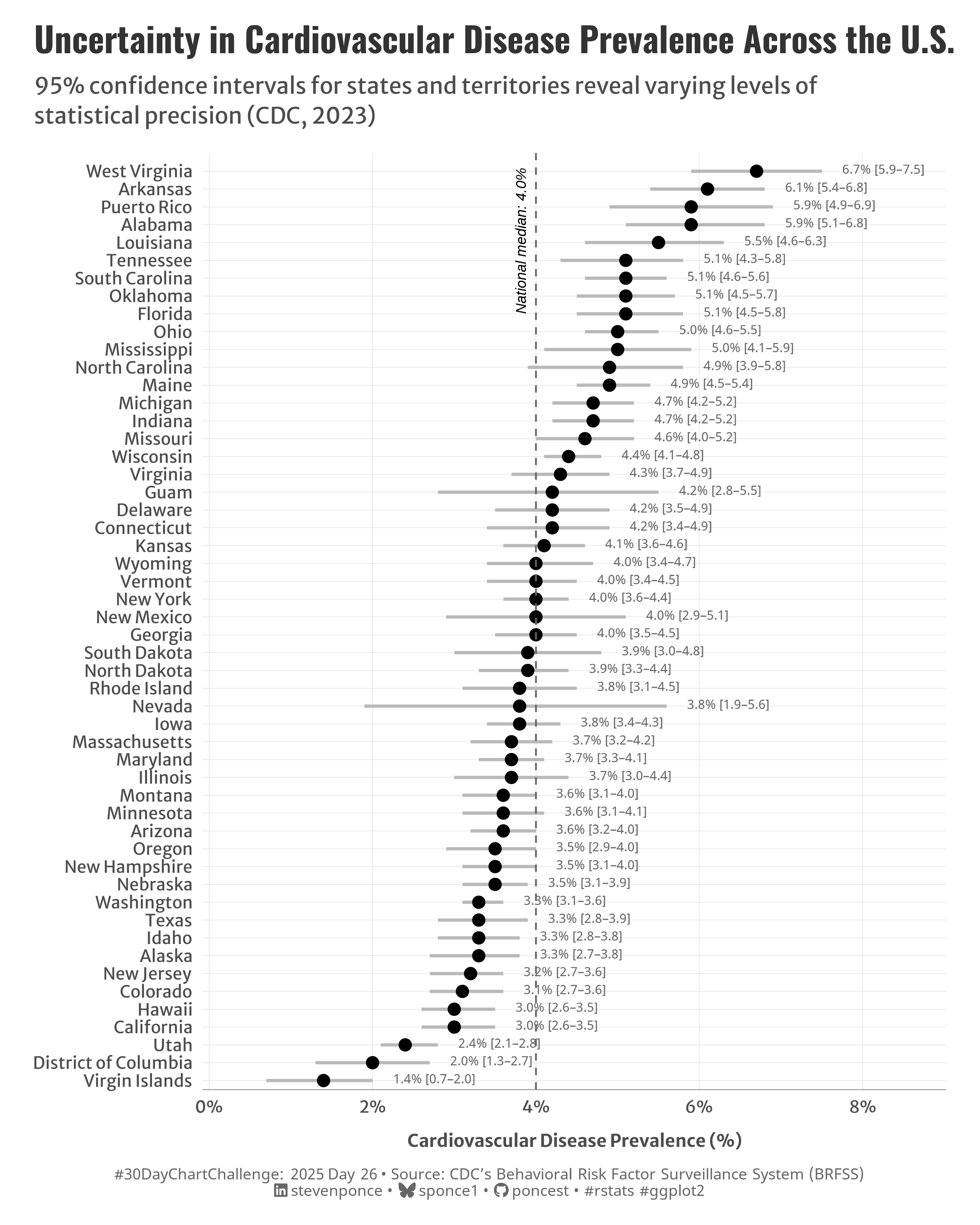{#fig-1}
### <mark> **Steps to Create this Graphic** </mark>
#### 1. Load Packages & Setup
```{r}
#| label: load
#| warning: false
#| message: false
#| results: "hide"
## 1. LOAD PACKAGES & SETUP ----
suppressPackageStartupMessages({
pacman::p_load(
  tidyverse,      # Easily Install and Load the 'Tidyverse'
  ggtext,         # Improved Text Rendering Support for 'ggplot2'
  showtext,       # Using Fonts More Easily in R Graphs
  janitor,        # Simple Tools for Examining and Cleaning Dirty Data
  skimr,          # Compact and Flexible Summaries of Data
  scales,         # Scale Functions for Visualization
  lubridate,      # Make Dealing with Dates a Little Easier
  ggrepel,        # Automatically Position Non-Overlapping Text Labels with 'ggplot2'
  camcorder       # Record Your Plot History
  )
})

### |- figure size ----
gg_record(
    dir    = here::here("temp_plots"),
    device = "png",
    width  = 8,
    height = 10,
    units  = "in",
    dpi    = 320
)

# Source utility functions
suppressMessages(source(here::here("R/utils/fonts.R")))
source(here::here("R/utils/social_icons.R"))
source(here::here("R/utils/image_utils.R"))
source(here::here("R/themes/base_theme.R"))
```
#### 2. Read in the Data
```{r}
#| label: read
#| include: true
#| eval: true
#| warning: false
cdc_prevalence_cardiovascular_disease <- read_csv(
  here::here(
    "data/Behavioral_Risk_Factor_Surveillance_System__BRFSS__Prevalence_Data__2011_to_present__20250409.csv")) |>
  clean_names()
```
#### 3. Examine the Data
```{r}
#| label: examine
#| include: true
#| eval: true
#| results: 'hide'
#| warning: false
glimpse(cdc_prevalence_cardiovascular_disease)
skim(cdc_prevalence_cardiovascular_disease)
```
#### 4. Tidy Data
```{r}
#| label: tidy
#| warning: false
### |- Tidy ----
# Prepare state-level data
state_cvd <- cdc_prevalence_cardiovascular_disease |>
  filter(year == 2023) |>
  filter(break_out == "Overall" | is.na(break_out)) |>
  filter(
    str_detect(locationdesc, "^[A-Z]") &
      !str_detect(locationdesc, "median|Median|average|Average")
  ) |>
  select(
    location = locationdesc,
    prevalence = data_value,
    lower_bound = confidence_limit_low,
    upper_bound = confidence_limit_high,
    sample_size,
    year
  ) |>
  mutate(
    ci_width = upper_bound - lower_bound,
    location = str_replace(location, " State$", ""),
    location = fct_reorder(location, prevalence)
  ) |>
  filter(!is.na(prevalence))

# Get national median estimate (US-level)
us_median <- cdc_prevalence_cardiovascular_disease |>
  filter(year == 2023, break_out == "Overall", locationabbr == "US") |>
  pull(data_value)
```
#### 5. Visualization Parameters
```{r}
#| label: params
#| include: true
#| warning: false
### |-  plot aesthetics ----
colors <- get_theme_colors(
  palette = c(
    "black", "gray40", "gray50", "gray70", "gray95", "white", "gray40"
    )
  )

### |-  titles and caption ----
# text
title_text    <- str_wrap("Uncertainty in Cardiovascular Disease Prevalence Across the U.S.",
                          width = 70)

subtitle_text <- str_wrap("95% confidence intervals for states and territories reveal varying levels of statistical precision (CDC, 2023)",
                          width = 80)

caption_text <- create_dcc_caption(
  dcc_year = 2025,
  dcc_day = 26,
  source_text =  "CDC’s Behavioral Risk Factor Surveillance System (BRFSS)"
)

### |-  fonts ----
setup_fonts()
fonts <- get_font_families()

### |-  plot theme ----

# Start with base theme
base_theme <- create_base_theme(colors)

# Add weekly-specific theme elements
weekly_theme <- extend_weekly_theme(
  base_theme,
  theme(

    # Text styling
    plot.title = element_text(face = "bold", family = fonts$title, size = rel(1.14), margin = margin(b = 10)),
    plot.subtitle = element_text(family = fonts$subtitle, color = colors$text, size = rel(0.78), margin = margin(b = 20)),

    # Axis elements
    axis.text = element_text(color = colors$text, size = rel(0.7)),
    axis.title.y = element_blank(),
    axis.title.x = element_text(color = colors$text, size = rel(0.8),
                                hjust = 0.5, margin = margin(t = 10)),

    axis.line.x = element_line(color = "gray50", linewidth = .2),

    # Grid elements
    panel.grid.minor.x = element_blank(),
    panel.grid.minor.y = element_blank(),
    panel.grid.major.y = element_line(color = "gray65", linewidth = 0.05),
    panel.grid.major.x = element_line(color = "gray65", linewidth = 0.05),

    # Plot margins
    plot.background = element_rect(fill = colors$palette[6], color = colors$palette[6]),
    panel.background = element_rect(fill = colors$palette[6], color = colors$palette[6]),
    plot.margin = margin(t = 10, r = 20, b = 10, l = 20),
  )
)

# Set theme
theme_set(weekly_theme)
```
#### 6. Plot
```{r}
#| label: plot
#| warning: false
### |-  Plot ----
p <- ggplot(state_cvd, aes(x = prevalence, y = location)) +
  # Geoms
  geom_segment(
    aes(x = lower_bound, xend = upper_bound, yend = location),
    color = colors$palette[4], linewidth = 0.9, alpha = 0.9
  ) +
  geom_point(
    size = 3, color = colors$palette[1],
    fill = colors$palette[1],
  ) +
  geom_text(
    aes(x = upper_bound, label = sprintf("%.1f%% [%.1f–%.1f]", prevalence, lower_bound, upper_bound)),
    nudge_x = 0.25, hjust = 0, vjust = 0.3, size = 2.7, color = colors$palette[2]
  ) +
  geom_vline(
    xintercept = us_median, color = colors$palette[2],
    linetype = "dashed", linewidth = 0.5
  ) +
  # Annotate
  annotate(
    "text", x = us_median, y = 44,
    label = sprintf("National median: %.1f%%", us_median),
    hjust = 0, vjust = -1, size = 3, color = colors$palette[1],
    fontface = "italic", angle = 90
  ) +
  # Scales
  scale_x_continuous(
    limits = c(0, max(state_cvd$upper_bound) + 0.7),
    labels = label_percent(scale = 1, suffix = "%"),
    breaks = seq(0, 8, by = 2),
    expand = expansion(mult = c(0.01, 0.1))
  ) +
  scale_y_discrete(
    expand = expansion(mult = c(0.01, 0.02))
  ) +
  # Labs
  labs(
    title = title_text,
    subtitle = subtitle_text,
    caption = caption_text,
    x = "Cardiovascular Disease Prevalence (%)",
    y = NULL
  ) +
  # Theme
  theme(
    plot.title = element_text(
      size = rel(1.45),
      family = fonts$title,
      face = "bold",
      color = colors$title,
      margin = margin(t = 5, b = 5)
    ),
    plot.subtitle = element_text(
      size = rel(0.95),
      family = fonts$subtitle,
      color = colors$subtitle,
      lineheight = 1.1,
      margin = margin(t = 5, b = 14)
    ),
    plot.caption = element_markdown(
      size = rel(0.65),
      family = fonts$caption,
      color = colors$caption,
      lineheight = 0.65,
      hjust = 0.5,
      halign = 0.5,
      margin = margin(t = 10, b = 5)
    ),
  )
```
#### 7. Save
```{r}
#| label: save
#| warning: false
### |-  plot image ----
save_plot(
  p,
  type = "30daychartchallenge",
  year = 2025,
  day = 26,
  width = 8,
  height = 10
  )
```
#### 8. Session Info
::: {.callout-tip collapse="true"}
##### Expand for Session Info
```{r, echo = FALSE}
#| eval: true
#| warning: false
sessionInfo()
```
:::
#### 9. GitHub Repository
::: {.callout-tip collapse="true"}
##### Expand for GitHub Repo
The complete code for this analysis is available in [`30dcc_2025_26.qmd`](https://github.com/poncest/personal-website/blob/master/data_visualizations/TidyTuesday/2025/30dcc_2025_26.qmd).
For the full repository, [click here](https://github.com/poncest/personal-website/).
:::
#### 10. References
::: {.callout-tip collapse="true"}
##### Expand for References
1. Data Sources:
- CDC’s Behavioral Risk Factor Surveillance System (BRFSS) [BRFSS: Prevalence of Cardiovascular Disease](https://data.cdc.gov/Behavioral-Risk-Factors/BRFSS-Graph-of-Current-Prevalence-of-Cardiovascula/gfhd-2f5y)
:::
