---
title: "S&P 500 Price Uncertainty and Noise"
subtitle: "Visualizing price trend, random variations, and forecast uncertainty"
description: "An exploration of market uncertainty and noise in S&P 500 price data, decomposing the signal from random variations and visualizing future prediction intervals with a fan chart."
date: "2025-04-27"
categories: ["30DayChartChallenge", "2025"]
tags: [
"financial-markets", "uncertainty-visualization", "time-series", "forecasting", "fan-charts", "noise-decomposition", "ggplot2", "quantmod", "signal-processing", "stock-market"
]
image: "thumbnails/30dcc_2025_27.png"
format:
html:
toc: true
toc-depth: 5
code-link: true
code-fold: true
code-tools: true
code-summary: "Show code"
editor_options:
chunk_output_type: inline
execute:
freeze: true
cache: true
error: false
message: false
warning: false
eval: true
# filters:
# - social-share
# share:
# permalink: "https://stevenponce.netlify.app/data_visualizations/30DayChartChallenge/2025/30dcc_2025_27.html"
# description: "Day 27 of #30DayChartChallenge: Visualizing uncertainties and noise in S&P 500 data with signal decomposition and forecast prediction intervals."
# twitter: true
# linkedin: true
# email: true
# facebook: false
# reddit: false
# stumble: false
# tumblr: false
# mastodon: true
# bsky: true
---
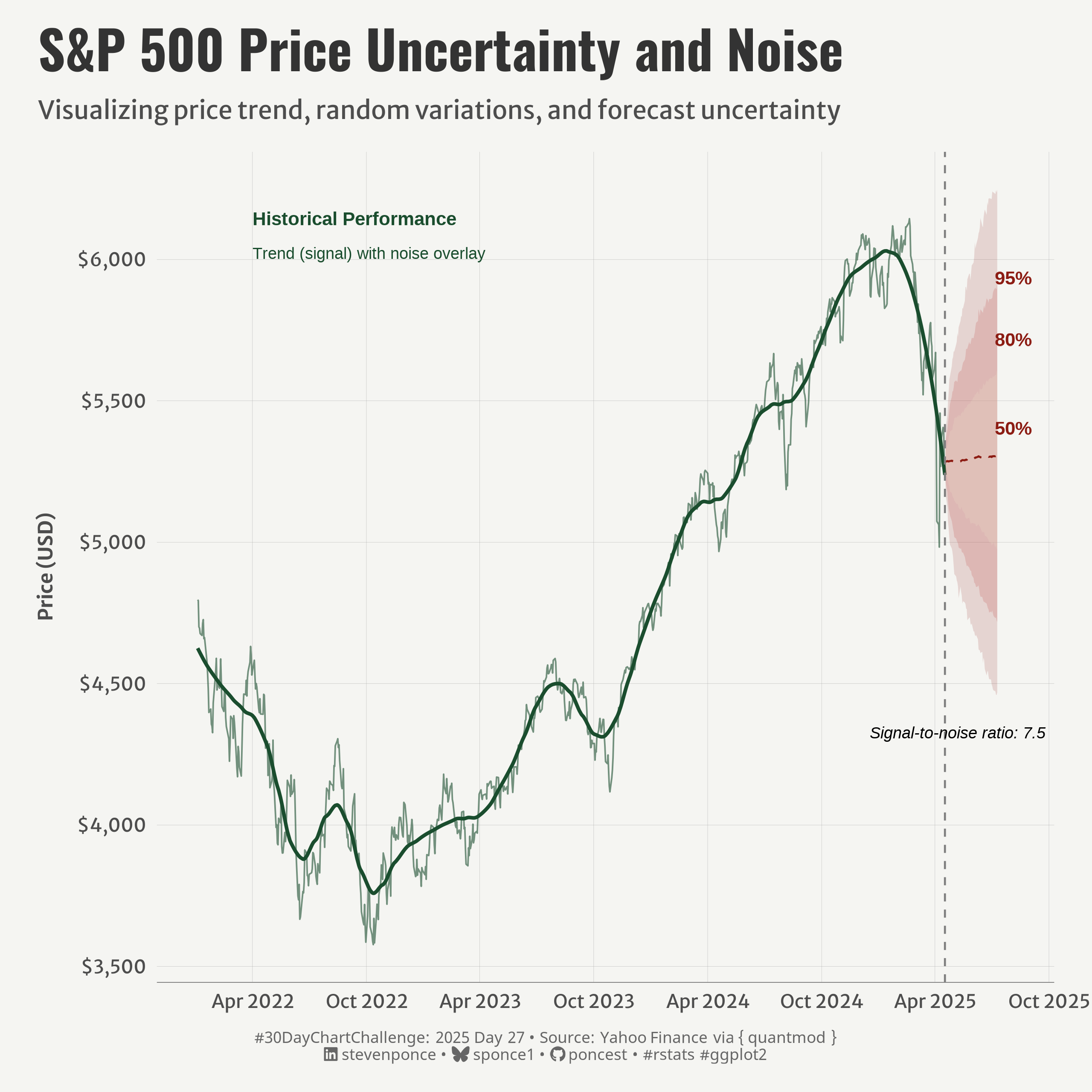{#fig-1}
### <mark> **Steps to Create this Graphic** </mark>
#### 1. Load Packages & Setup
```{r}
#| label: load
#| warning: false
#| message: false
#| results: "hide"
## 1. LOAD PACKAGES & SETUP ----
suppressPackageStartupMessages({
pacman::p_load(
  tidyverse,      # Easily Install and Load the 'Tidyverse'
  ggtext,         # Improved Text Rendering Support for 'ggplot2'
  showtext,       # Using Fonts More Easily in R Graphs
  janitor,        # Simple Tools for Examining and Cleaning Dirty Data
  skimr,          # Compact and Flexible Summaries of Data
  scales,         # Scale Functions for Visualization
  lubridate,      # Make Dealing with Dates a Little Easier
  ggrepel,        # Automatically Position Non-Overlapping Text Labels with 'ggplot2'
  quantmod,       # Quantitative Financial Modelling Framework
  camcorder       # Record Your Plot History
  )
})

### |- figure size ----
gg_record(
    dir    = here::here("temp_plots"),
    device = "png",
    width  = 8,
    height = 8,
    units  = "in",
    dpi    = 320
)

# Source utility functions
suppressMessages(source(here::here("R/utils/fonts.R")))
source(here::here("R/utils/social_icons.R"))
source(here::here("R/utils/image_utils.R"))
source(here::here("R/themes/base_theme.R"))
```
#### 2. Read in the Data
```{r}
#| label: read
#| include: true
#| eval: true
#| warning: false
# Get S&P 500 data (just last 2 years to keep it faster)
getSymbols("^GSPC", from = "2022-01-01")
# Convert to data frame and prepare data
sp500_df <- GSPC |>
  as.data.frame() |>
  rownames_to_column(var = "date") |>
  mutate(date = as.Date(date)) |>
  select(date, GSPC.Adjusted) |>
  rename(price = GSPC.Adjusted)
```
#### 3. Examine the Data
```{r}
#| label: examine
#| include: true
#| eval: true
#| results: 'hide'
#| warning: false
glimpse(sp500_df)
skim(sp500_df)
```
#### 4. Tidy Data
```{r}
#| label: tidy
#| warning: false
### |- Tidy ----
# Calculate log returns
sp500_df <- sp500_df |>
  arrange(date) |>
  mutate(log_return = c(NA, diff(log(price))))

# Decompose the signal into trend and noise components
# Use loess smoothing to extract the trend
loess_fit <- loess(price ~ as.numeric(date), data = sp500_df, span = 0.15)
sp500_df$trend <- predict(loess_fit)
sp500_df$noise <- sp500_df$price - sp500_df$trend

# Calculate noise metrics
noise_sd <- sd(sp500_df$noise, na.rm = TRUE)
noise_range <- max(sp500_df$noise, na.rm = TRUE) - min(sp500_df$noise, na.rm = TRUE)
signal_to_noise <- sd(sp500_df$trend, na.rm = TRUE) / noise_sd

# Calculate historical volatility (standard deviation of returns)
vol <- sd(sp500_df$log_return, na.rm = TRUE)

# Create forecast data
last_date <- max(sp500_df$date)
last_price <- sp500_df |> filter(date == last_date) |> pull(price)
forecast_days <- 60

# Create date sequence for weekdays only
all_dates <- seq.Date(from = last_date + days(1),
                      by = "day",
                      length.out = forecast_days * 1.5) # Add buffer for weekends
forecast_dates <- all_dates[!weekdays(all_dates) %in% c("Saturday", "Sunday")]
forecast_dates <- head(forecast_dates, forecast_days)

# Simple random walk simulation for forecasting
set.seed(123)
n_simulations <- 1000
simulations <- matrix(nrow = length(forecast_dates), ncol = n_simulations)

for (i in 1:n_simulations) {
  # Start with last known price
  price <- last_price
  # Generate random returns based on historical volatility
  random_returns <- rnorm(length(forecast_dates), mean = 0, sd = vol)

  for (j in 1:length(forecast_dates)) {
    # Apply random return
    price <- price * exp(random_returns[j])
    simulations[j, i] <- price
  }
}

# Calculate percentiles for confidence intervals
forecast_df <- data.frame(
  date = forecast_dates,
  mean = rowMeans(simulations),
  lower_95 = apply(simulations, 1, quantile, probs = 0.025),
  lower_80 = apply(simulations, 1, quantile, probs = 0.1),
  lower_50 = apply(simulations, 1, quantile, probs = 0.25),
  upper_50 = apply(simulations, 1, quantile, probs = 0.75),
  upper_80 = apply(simulations, 1, quantile, probs = 0.9),
  upper_95 = apply(simulations, 1, quantile, probs = 0.975)
)
```
#### 5. Visualization Parameters
```{r}
#| label: params
#| include: true
#| warning: false
### |-  plot aesthetics ----
colors <- get_theme_colors(
  palette = c(
    "#8C1C13", "#BF4342", "#E7D7C1", "#1A4D2E"
    )
  )

### |-  titles and caption ----
# text
title_text    <- str_wrap("S&P 500 Price Uncertainty and Noise",
                          width = 70)

subtitle_text <- str_wrap("Visualizing price trend, random variations, and forecast uncertainty",
                          width = 80)

caption_text <- create_dcc_caption(
  dcc_year = 2025,
  dcc_day = 27,
  source_text =  "Yahoo Finance via { quantmod }"
)

### |-  fonts ----
setup_fonts()
fonts <- get_font_families()

### |-  plot theme ----

# Start with base theme
base_theme <- create_base_theme(colors)

# Add weekly-specific theme elements
weekly_theme <- extend_weekly_theme(
  base_theme,
  theme(

    # Text styling
    plot.title = element_text(face = "bold", family = fonts$title, size = rel(1.14), margin = margin(b = 10)),
    plot.subtitle = element_text(family = fonts$subtitle, color = colors$text, size = rel(0.78), margin = margin(b = 20)),

    # Axis elements
    axis.text = element_text(color = colors$text, size = rel(0.7)),
    axis.title.y = element_text(color = colors$text, size = rel(0.8),
                                hjust = 0.5, margin = margin(r = 10)),
    axis.title.x = element_text(color = colors$text, size = rel(0.8),
                                hjust = 0.5, margin = margin(t = 10)),

    axis.line.x = element_line(color = "gray50", linewidth = .2),

    # Grid elements
    panel.grid.minor.x = element_blank(),
    panel.grid.minor.y = element_blank(),
    panel.grid.major.y = element_line(color = "gray65", linewidth = 0.05),
    panel.grid.major.x = element_line(color = "gray65", linewidth = 0.05),

    # Plot margins
    plot.margin = margin(t = 10, r = 20, b = 10, l = 20),
  )
)

# Set theme
theme_set(weekly_theme)
```
#### 6. Plot
```{r}
#| label: plot
#| warning: false
### |-  Plot ----
p <- ggplot() +
  # Geom
  geom_line( # tend line
    data = sp500_df, aes(x = date, y = trend),
    color = colors$palette[4], linewidth = 0.9
    ) +
  geom_line( # noise around trend
    data = sp500_df, aes(x = date, y = price),
    color = colors$palette[4], linewidth = 0.4, alpha = 0.6
    ) +
  geom_ribbon(
    data = forecast_df,  # 95% prediction interval
    aes(x = date, ymin = lower_95, ymax = upper_95),
    fill = colors$palette[1], alpha = 0.15
    ) +
  geom_ribbon(
    data = forecast_df,  # 80% prediction interval
    aes(x = date, ymin = lower_80, ymax = upper_80),
    fill = colors$palette[2], alpha = 0.2
    ) +
  geom_ribbon(
    data = forecast_df,  # 50% prediction interval
    aes(x = date, ymin = lower_50, ymax = upper_50),
    fill = colors$palette[3], alpha = 0.3,
    ) +
  geom_line(
    data = forecast_df,  # Mean forecast
    aes(x = date, y = mean),
    color = colors$palette[1], linetype = "dashed", linewidth = 0.5
    ) +
   geom_vline(
    xintercept = as.numeric(last_date),
    linetype = "dashed", color = "gray50"
    ) +
  # Annotation
  annotate(
    "text", x = as.Date("2022-04-01"), y = max(sp500_df$price),
           label = "Historical Performance", hjust = 0,
           fontface = "bold", color = colors$palette[4], size = 3.5
    ) +
  annotate(
    "text", x = as.Date("2022-04-01"), y = max(sp500_df$price) * 0.98,
    label = paste0("Trend (signal) with noise overlay"),
    hjust = 0, color = colors$palette[4], size = 3
    ) +
  annotate(
    "text", x = last_date + days(110), y = max(forecast_df$upper_95) * 0.95,
    label = "95%", color = colors$palette[1], fontface = "bold", size = 3.5
    ) +
  annotate(
    "text", x = last_date + days(110), y = max(forecast_df$upper_80),
    label = "80%", color = colors$palette[1], fontface = "bold", size = 3.5,
    vjust = 5
    ) +
  annotate(
    "text", x = last_date + days(110), y = max(forecast_df$upper_50),
    label = "50%", color = colors$palette[1], fontface = "bold", size = 3.5,
    vjust = 5
    ) +
  annotate(
    "text", x = forecast_dates[length(forecast_dates)/4], y = min(forecast_df$lower_95) * 0.97,
    label = paste0("Signal-to-noise ratio: ", round(signal_to_noise, 1)),
    hjust = 0.5, fontface = "italic", size = 3
    ) +
  # Scales
  scale_y_continuous(
    labels = scales::dollar_format()
    ) +
  scale_x_date(
    date_breaks = "6 months", date_labels = "%b %Y"
    ) +
  # Labs
  labs(
    title = title_text,
    subtitle = subtitle_text,
    caption = caption_text,
    x = NULL,
    y = "Price (USD)",
  ) +
  # Theme
  theme(
    plot.title = element_text(
      size = rel(2),
      family = fonts$title,
      face = "bold",
      color = colors$title,
      margin = margin(t = 5, b = 5)
    ),
    plot.subtitle = element_text(
      size = rel(0.95),
      family = fonts$subtitle,
      color = colors$subtitle,
      lineheight = 1.1,
      margin = margin(t = 5, b = 14)
    ),
    plot.caption = element_markdown(
      size = rel(0.6),
      family = fonts$caption,
      color = colors$caption,
      lineheight = 0.65,
      hjust = 0.5,
      halign = 0.5,
      margin = margin(t = 10, b = 5)
    ),
  )
```
#### 7. Save
```{r}
#| label: save
#| warning: false
### |-  plot image ----
save_plot(
  p,
  type = "30daychartchallenge",
  year = 2025,
  day = 27,
  width = 8,
  height = 8
  )
```
#### 8. Session Info
::: {.callout-tip collapse="true"}
##### Expand for Session Info
```{r, echo = FALSE}
#| eval: true
#| warning: false
sessionInfo()
```
:::
#### 9. GitHub Repository
::: {.callout-tip collapse="true"}
##### Expand for GitHub Repo
The complete code for this analysis is available in [`30dcc_2025_27.qmd`](https://github.com/poncest/personal-website/blob/master/data_visualizations/TidyTuesday/2025/30dcc_2025_27.qmd).
For the full repository, [click here](https://github.com/poncest/personal-website/).
:::
#### 10. References
::: {.callout-tip collapse="true"}
##### Expand for References
1. Data Sources:
- Yahoo Finance via { quantmod } [quantmod](https://www.quantmod.com/)
:::
