---
title: "THE HIDDEN UNCERTAINTY"
subtitle: "Mapping measurement challenges in Alaska's vanishing glaciers"
description: "An exploration of measurement uncertainty in Alaska's glaciers from 1946-2023, visualized in National Geographic style. This visualization reveals how distance from observation points, glacier size, and remote locations contribute to measurement challenges in tracking glacier changes across different Alaskan regions."
date: "2025-04-30"
categories: ["30DayChartChallenge", "2025"]
tags: [
"Uncertainties",
"National Geographic",
"Glaciers",
"Climate Science",
"Spatial Analysis",
"Error Estimation",
"ggplot2",
"Alaska",
"Scientific Visualization",
"Environmental Data"
]
image: "thumbnails/30dcc_2025_30.png"
format:
html:
toc: true
toc-depth: 5
code-link: true
code-fold: true
code-tools: true
code-summary: "Show code"
editor_options:
chunk_output_type: inline
execute:
freeze: true
cache: true
error: false
message: false
warning: false
eval: true
# filters:
# - social-share
# share:
# permalink: "https://stevenponce.netlify.app/data_visualizations/30DayChartChallenge/2025/30dcc_2025_30.html"
# description: "Day 30 of #30DayChartChallenge: Visualizing the hidden uncertainty in Alaska's glacier measurements with National Geographic styling #DataViz #RStats #ClimateScience"
# twitter: true
# linkedin: true
# email: true
# facebook: false
# reddit: false
# stumble: false
# tumblr: false
# mastodon: true
# bsky: true
---
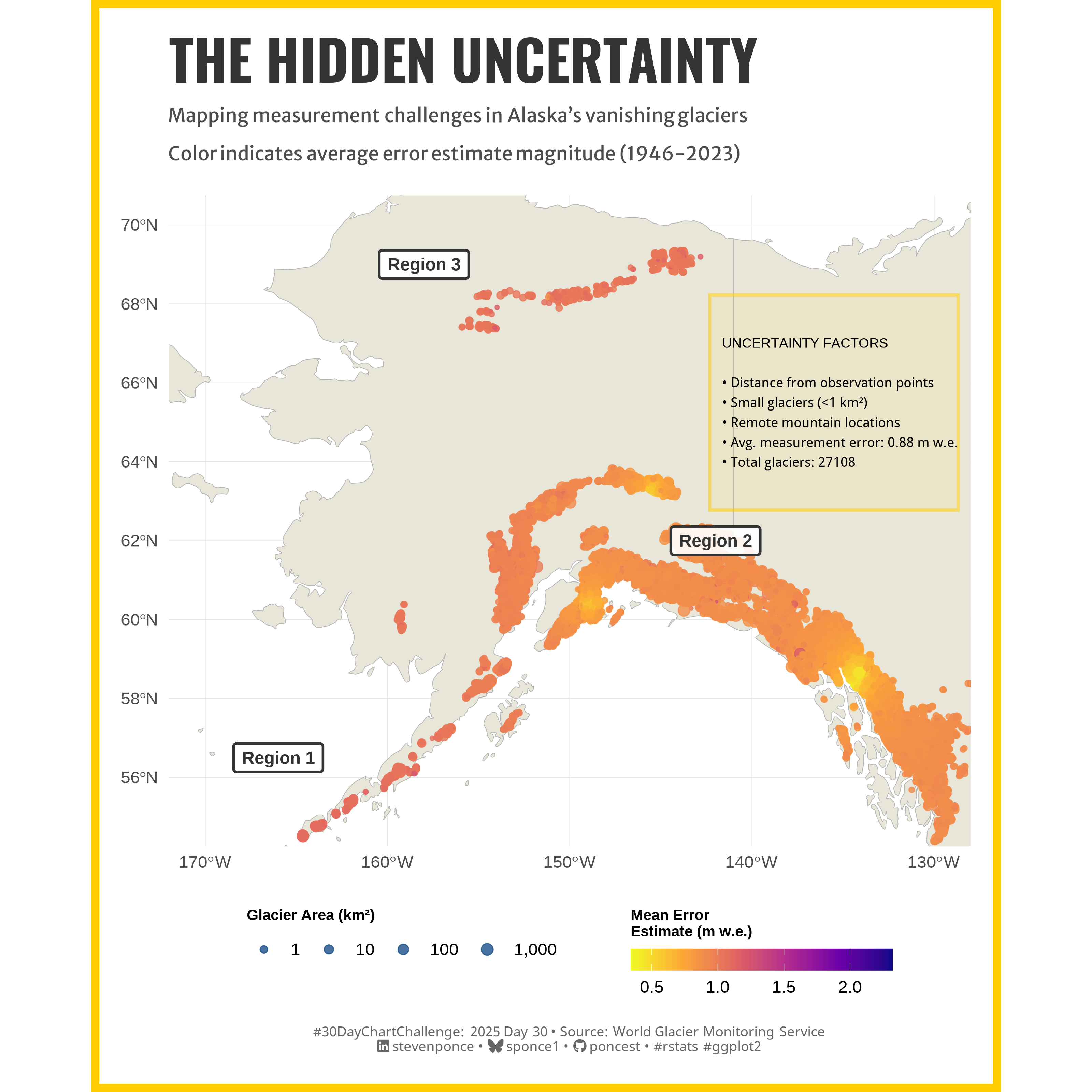{#fig-1}
### <mark> **Steps to Create this Graphic** </mark>
#### 1. Load Packages & Setup
```{r}
#| label: load
#| warning: false
#| message: false
#| results: "hide"
## 1. LOAD PACKAGES & SETUP ----
suppressPackageStartupMessages({
pacman::p_load(
  tidyverse,          # Easily Install and Load the 'Tidyverse'
  ggtext,             # Improved Text Rendering Support for 'ggplot2'
  showtext,           # Using Fonts More Easily in R Graphs
  janitor,            # Simple Tools for Examining and Cleaning Dirty Data
  skimr,              # Compact and Flexible Summaries of Data
  scales,             # Scale Functions for Visualization
  lubridate,          # Make Dealing with Dates a Little Easier
  ggdist,             # Visualizations of Distributions and Uncertainty
  sf,                 # Simple Features for R
  rnaturalearth,      # World Map Data from Natural Earth
  rnaturalearthdata,  # World Vector Map Data from Natural Earth Used in 'rnaturalearth'
  viridis,            # Colorblind-Friendly Color Maps for R
  ggnewscale,         # Multiple Fill and Colour Scales in 'ggplot2'
  ggrepel,            # Automatically Position Non-Overlapping Text Labels with 'ggplot2'
  camcorder       # Record Your Plot History
  )
})

### |- figure size ----
gg_record(
    dir    = here::here("temp_plots"),
    device = "png",
    width  = 10,
    height = 10,
    units  = "in",
    dpi    = 320
)

# Source utility functions
suppressMessages(source(here::here("R/utils/fonts.R")))
source(here::here("R/utils/social_icons.R"))
source(here::here("R/utils/image_utils.R"))
source(here::here("R/themes/base_theme.R"))
```
#### 2. Read in the Data
```{r}
#| label: read
#| include: true
#| eval: true
#| warning: false
alaska_combined <- readRDS(
  here::here(
    "data/30DayChartChallenge/2025/alaska_combined_data.rds")) |>
  clean_names()
```
#### 3. Examine the Data
```{r}
#| label: examine
#| include: true
#| eval: true
#| results: 'hide'
#| warning: false
glimpse(alaska_combined)
skim(alaska_combined)
```
#### 4. Prep Data
> For the data preparation step, refer to the [`data_preparation.R`](https://github.com/poncest/30DayChartChallenge/blob/main/2025/day_30/data_preparation.R) file in my GitHub repository.
#### 4.1 Tidy Data
```{r}
#| label: tidy
#| warning: false
### |- Tidy ----
# Base map data
world <- ne_countries(scale = "medium", returnclass = "sf")
alaska_bounds <- st_bbox(c(
  xmin = -170, ymin = 55, xmax = -130, ymax = 70), crs = st_crs(4326)
  )

# Calculate average error per glacier over all years
glacier_avg_error <- alaska_combined |>
  group_by(rgi_id, region, cen_lon, cen_lat, area) |>
  summarize(
    mean_error = mean(error_estimate, na.rm = TRUE),
    mean_dist = mean(mean_dist_gla_anom, na.rm = TRUE),
    .groups = "drop"
  )

# Convert to SF for mapping
glacier_error_sf <- glacier_avg_error |>
  st_as_sf(coords = c("cen_lon", "cen_lat"), crs = 4326)

# Define regions
region_points <- tibble(
  region_id = c("Region 1", "Region 2", "Region 3"),
  lon = c(-166, -142, -158),
  lat = c(56.5, 62, 69),
  color = c("gray20", "gray20", "gray20")
)

# Convert to SF for plotting
region_points_sf <- st_as_sf(
  region_points, coords = c("lon", "lat"), crs = 4326
  )

# Create informational box
# Extract uncertainty statistics
uncertainty_stats <- glacier_avg_error |>
  summarize(
    mean_error = mean(mean_error, na.rm = TRUE),
    max_error = max(mean_error, na.rm = TRUE),
    min_error = min(mean_error, na.rm = TRUE),
    glacier_count = n()
  )

# Textbox
info_box_text <- paste0(
  "UNCERTAINTY FACTORS\n\n",
  "• Distance from observation points\n",
  "• Small glaciers (<1 km²)\n",
  "• Remote mountain locations\n",
  "• Avg. measurement error: ", round(uncertainty_stats$mean_error, 2), " m w.e.\n",
  "• Total glaciers: ", uncertainty_stats$glacier_count
)
```
#### 5. Visualization Parameters
```{r}
#| label: params
#| include: true
#| warning: false
### |-  plot aesthetics ----
colors <- get_theme_colors(
  palette = c(
    "water" = "#71ABD8",
    "land" = "#E8E6D9",
    "glacier" = "#D1E6EC",
    "highlight" = "#FFCD00",
    "text" = "#000000",
    "uncertainty" = "#8BB9DD",
    "dark_blue" = "#1A5088",
    "text_gray" = "#555555"
    )
  )

### |-  titles and caption ----
# text
title_text    <- str_glue("THE HIDDEN UNCERTAINTY")

subtitle_text <- str_glue("Mapping measurement challenges in Alaska's vanishing glaciers\n
                          Color indicates average error estimate magnitude (1946-2023)")

caption_text <- create_dcc_caption(
  dcc_year = 2025,
  dcc_day = 30,
  source_text =  "World Glacier Monitoring Service"
)

### |-  fonts ----
setup_fonts()
fonts <- get_font_families()

### |-  plot theme ----

# National Geographic theme (at least my interpretation)
theme_natgeo <- function() {
  theme_minimal(base_size = 14) +
    theme(
      # Text elements
      plot.title = element_text(face = "bold", size = 20, family = "sans"),
      plot.subtitle = element_text(size = 14, family = "sans", margin = margin(b = 20)),
      axis.title = element_text(face = "bold", size = 10),
      legend.title = element_text(face = "bold", size = 10),

      # Grid elements
      panel.grid.major = element_line(color = "gray90", size = 0.2),
      panel.grid.minor = element_blank(),

      # Background elements
      plot.background = element_rect(fill = "white", color = NA),
      panel.background = element_rect(fill = "white", color = NA),

      # Margins and spacing
      plot.margin = margin(20, 20, 20, 20),
      legend.margin = margin(10, 10, 10, 10),

      # Caption styling
      plot.caption = element_text(size = 9, hjust = 0, color = colors$palette["text_gray"],
                                  margin = margin(t = 15))
    )
}
```
#### 6. Plot
```{r}
#| label: plot
#| warning: false
### |-  Plot ----
# Main map -----
main_map <- ggplot() +
  # Base map
  geom_sf(data = world, fill = colors$palette['land'], color = "gray70") +

  # Geoms
  geom_sf(
    data = glacier_error_sf,
    aes(size = area, color = mean_error),
    alpha = 0.8
    ) +
  geom_label(
    data = region_points_sf,
    aes(geometry = geometry, label = region_id),
    stat = "sf_coordinates",
    fill = "white",
    color = region_points$color,
    fontface = "bold",
    size = 4,
    label.padding = unit(0.4, "lines"),
    label.r = unit(0.15, "lines"),
    alpha = 0.9,
    label.size = 0.8
  ) +
  # Scales
  scale_color_viridis_c(
    name = "Mean Error\nEstimate (m w.e.)",
    option = "plasma",
    direction = -1,
    guide = guide_colorbar(
      title.position = "top",
      barwidth = 12,
      barheight = 1
    )
  ) +
  scale_size_continuous(
    name = "Glacier Area (km²)",
    range = c(0.1, 3.5),
    breaks = c(1, 10, 100, 1000),
    trans = "log10",
    labels = label_comma(),
    guide = guide_legend(
      title.position = "top",
      override.aes = list(color = colors$palette["dark_blue"])
    )
  ) +
  coord_sf(  # Alaska region
    xlim = c(alaska_bounds$xmin, alaska_bounds$xmax),
    ylim = c(alaska_bounds$ymin, alaska_bounds$ymax)
  ) +
  # Labs
  labs(
    title = title_text,
    subtitle = subtitle_text,
    caption = caption_text,
    x = NULL,
    y = NULL
  ) +
  # Theme
  theme_natgeo() +
  theme(

    legend.position = "bottom",
    legend.box = "horizontal",
    legend.direction = "horizontal",
    legend.spacing.x = unit(1, "cm"),
    legend.box.spacing = unit(0.5, "cm"),
    legend.key.size = unit(0.8, "cm"),

    plot.title = element_text(
      size = rel(2.6),
      family = fonts$title,
      face = "bold",
      color = colors$title,
      margin = margin(t = 5, b = 5)
    ),
    plot.subtitle = element_markdown(
      size = rel(0.90),
      family = fonts$subtitle,
      color = colors$subtitle,
      lineheight = 0.8,
      margin = margin(t = 5, b = 20)
    ),
    plot.caption = element_markdown(
      size = rel(0.65),
      family = fonts$caption,
      color = colors$caption,
      lineheight = 0.65,
      hjust = 0.5,
      halign = 0.5,
      margin = margin(t = 10, b = 5)
    ),
  )

# Info textbox -----
info_box <- ggplot() +
  annotate(
    "rect",
    xmin = 0, xmax = 1, ymin = 0, ymax = 1,
    fill = alpha(colors$palette["highlight"], 0.08)
  ) +
  annotate(
    "text",
    x = 0.05, y = 0.5,
    label = info_box_text,
    hjust = 0, vjust = 0.5,
    size = 3.2,
    fontface = "plain",
    color = colors$palette["text"]
  ) +
  annotate(
    "rect",
    xmin = 0, xmax = 1, ymin = 0, ymax = 1,
    fill = NA, color = alpha(colors$palette["highlight"], 0.5),
    linewidth = 1
  ) +
  theme_void() +
  xlim(0, 1) + ylim(0, 1)

# Combine main map and info box -----
combined_map <- main_map +
  annotation_custom(
    grob = ggplotGrob(info_box),
    xmin = -143, xmax = -128,
    ymin = 62.5, ymax = 68.5
  )

# Final map -----
final_map <- combined_map +
  theme(
    plot.background = element_rect(
      fill = "white",
      color = colors$palette["highlight"],
      linewidth = 5
    )
  )
```
#### 7. Save
```{r}
#| label: save
#| warning: false
### |-  plot image ----
save_plot(
  final_map,
  type = "30daychartchallenge",
  year = 2025,
  day = 30,
  width = 10,
  height = 10
  )
```
#### 8. Session Info
::: {.callout-tip collapse="true"}
##### Expand for Session Info
```{r, echo = FALSE}
#| eval: true
#| warning: false
sessionInfo()
```
:::
#### 9. GitHub Repository
::: {.callout-tip collapse="true"}
##### Expand for GitHub Repo
The complete code for this analysis is available in [`30dcc_2025_30.qmd`](https://github.com/poncest/personal-website/blob/master/data_visualizations/TidyTuesday/2025/30dcc_2025_30.qmd).
For the full repository, [click here](https://github.com/poncest/personal-website/).
:::
#### 10. References
::: {.callout-tip collapse="true"}
##### Expand for References
1. Data Sources:
- Dussaillant, I., Hugonnet, R., Huss, M., Berthier, E., Bannwart, J., Paul, F., and Zemp, M. (2025): Annual mass-change estimates for the world’s glaciers. [glacier time series and gridded data products.](https://doi.org/10.5904/wgms-amce-2025-02)
:::
