---
title: "Britain's Power Mix: A Daily Energy Snapshot"
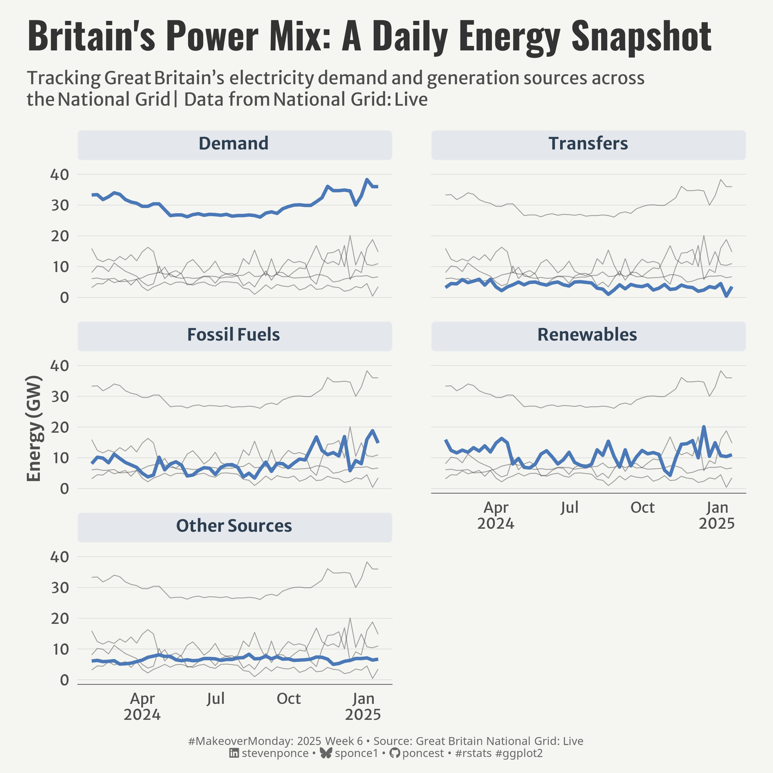
subtitle: "Tracking Great Britain's electricity demand and generation sources across the National Grid | Data from National Grid: Live"
description: "Analysis of Britain's electricity network through small multiples visualization, showing daily patterns in energy demand, generation sources, and transfers. The visualization explores the interplay between different power sources across the National Grid from April 2024 to January 2025."
author: "Steven Ponce"
date: "2025-02-02"
categories: ["MakeoverMonday", "2025"]
tags: [
"ggplot2",
"tidyverse",
"energy-data",
"time-series",
"small-multiples",
"national-grid",
"electricity",
"britain",
"power-generation",
"renewable-energy",
"fossil-fuels",
"data-journalism",
"energy-analytics"
]
image: "thumbnails/mm_2025_06.png"
format:
html:
toc: true
toc-depth: 5
code-link: true
code-fold: true
code-tools: true
code-summary: "Show code"
editor_options:
chunk_output_type: inline
execute:
freeze: true
cache: true
error: false
message: false
warning: false
eval: true
# filters:
# - social-share
# share:
# permalink: "https://stevenponce.netlify.app/data_visualizations/MakeoverMonday/2025/mm_2025_06.html"
# description: "Exploring Britain's daily energy patterns: A visualization of power demand, renewable and fossil fuel generation, and grid transfers across the National Grid system #DataViz #MakeoverMonday #EnergyData"
# twitter: true
# linkedin: true
# email: true
# facebook: false
# reddit: false
# stumble: false
# tumblr: false
# mastodon: true
# bsky: true
---
### Original
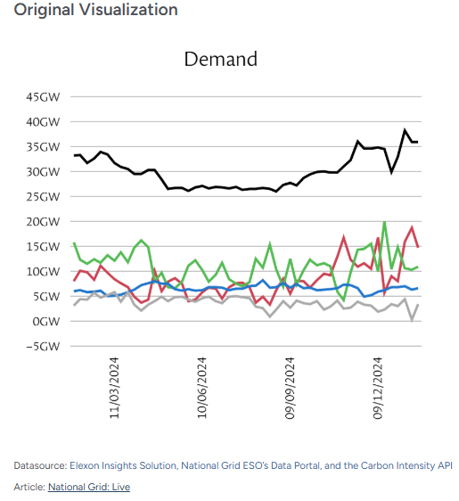
The original visualization comes from the National Grid: Live (The National Grid is the electric power transmission network for Great Britain).
`
Source: [Elexon Insights Solution, National Grid ESO’s Data Portal, and the Carbon Intensity API](https://grid.iamkate.com/)
### Makeover
{#fig-1}
### <mark> **Steps to Create this Graphic** </mark>
#### 1. Load Packages & Setup
```{r}
#| label: load
#| warning: false
#| message: false
#| results: "hide"
## 1. LOAD PACKAGES & SETUP ----
suppressPackageStartupMessages({
pacman::p_load(
tidyverse,      # Easily Install and Load the 'Tidyverse'
   tidyverse,      # Easily Install and Load the 'Tidyverse'
    ggtext,         # Improved Text Rendering Support for 'ggplot2'
    showtext,       # Using Fonts More Easily in R Graphs
    janitor,        # Simple Tools for Examining and Cleaning Dirty Data
    skimr,          # Compact and Flexible Summaries of Data
    scales,         # Scale Functions for Visualization
    glue,           # Interpreted String Literals
    here,           # A Simpler Way to Find Your Files
    lubridate,      # Make Dealing with Dates a Little Easier
    camcorder,      # Record Your Plot History
    patchwork,      # The Composer of Plots
    gghighlight     # Highlight Lines and Points in 'ggplot2'
)
})

### |- figure size ----
gg_record(
    dir    = here::here("temp_plots"),
    device = "png",
    width  =  8,
    height =  8,
    units  = "in",
    dpi    = 320
)

# Source utility functions
suppressMessages(source(here::here("R/utils/fonts.R")))
source(here::here("R/utils/social_icons.R"))
source(here::here("R/utils/image_utils.R"))
source(here::here("R/themes/base_theme.R"))
```
#### 2. Read in the Data
```{r}
#| label: read
#| include: true
#| eval: true
#| warning: false
energy_raw <- read_csv(
  here::here('data/National_Grid_Energy_Breakdown.csv')) |>
  clean_names()
```
#### 3. Examine the Data
```{r}
#| label: examine
#| include: true
#| eval: true
#| results: 'hide'
#| warning: false
glimpse(energy_raw)
skim(energy_raw)
```
#### 4. Tidy Data
```{r}
#| label: tidy
#| warning: false
### |-  tidy data ----
energy_clean <- energy_raw |>
  rename_with(~str_remove(., pattern = "_gw"), everything()) |>
  mutate(date = dmy(date)) |>
  # Pivot longer
  pivot_longer(
    cols = !date,
    names_to = "metric",
    values_to = "demand_gw"
  ) |>
  mutate(
    metric = case_when(
      metric == "fossil_fuels" ~ "fossil fuels",
      metric == "other_sources" ~ "other sources",
      TRUE ~ metric
    ),
    metric = str_to_title(metric),
    metric = factor(metric,
                    levels = c("Demand",
                               "Transfers",
                               "Fossil Fuels",
                               "Renewables",
                               "Other Sources")
    )
  )
```
#### 5. Visualization Parameters
```{r}
#| label: params
#| include: true
#| warning: false
### |-  plot aesthetics ----
# Get base colors with custom palette
colors <- get_theme_colors(palette = c("#4B79B7", "#F8F9FA", "#2C3E50", "#34495E", "#7F8C8D"))

### |-  titles and caption ----
title_text <- str_glue("Britain's Power Mix: A Daily Energy Snapshot")
subtitle_text <- str_glue("Tracking Great Britain's electricity demand and generation sources across<br>
                          the National Grid | Data from National Grid: Live")

# Create caption
caption_text <- create_mm_caption(
    mm_year = 2025,
    mm_week = 06,
    source_text = "Great Britain National Grid: Live"
)

### |-  fonts ----
setup_fonts()
fonts <- get_font_families()

### |-  plot theme ----

# Start with base theme
base_theme <- create_base_theme(colors)

# Add weekly-specific theme elements
weekly_theme <- extend_weekly_theme(
  base_theme,
  theme(
    # Weekly-specific modifications
    axis.line.x           = element_line(color = "#252525", linewidth = .2),

    panel.spacing.x       = unit(2, 'lines'),
    panel.spacing.y       = unit(1, 'lines'),
    panel.grid.major.x    = element_blank(),
    panel.grid.major.y    = element_line(color = alpha(colors[5], 0.2), linewidth = 0.2),
    panel.grid.minor      = element_blank(),

    strip.text          = element_textbox(
      size              = rel(0.9),
      face              = 'bold',
      color             = colors$palette[3],
      fill              = alpha(colors$palette[1], 0.1),
      box.color         = alpha(colors[1], 0.5),
      halign            = 0.5,
      linetype          = 1,
      r                 = unit(3, "pt"),
      width             = unit(1, "npc"),
      padding           = margin(5, 10, 5, 10),
      margin            = margin(b = 10)
    ),
  )
)

# Set theme
theme_set(weekly_theme)
```
#### 6. Plot
```{r}
#| label: plot
#| warning: false
### |-  Plot  ----
p <- ggplot(energy_clean,
       aes(x = date, y = demand_gw, group = metric)) +
  # Geoms
  geom_line(linewidth = 0.3, alpha = 0.2) +
  gghighlight(
    use_direct_label = FALSE,
    unhighlighted_params = list(
      linewidth = 0.3,
      alpha = 0.45,
      color = 'gray20'
    )
  ) +
  geom_line(color = colors$palette[1], linewidth = 1.2) +

  # Scales
  scale_x_date(
    breaks = "3 month",
    labels = label_date_short(),
    limits = c(min(energy_clean$date), max(energy_clean$date))
  ) +
  scale_y_continuous(breaks = pretty_breaks()) +
  coord_cartesian(clip = 'off') +

  # Labs
  labs(
    x = NULL,
    y = "Energy (GW)",
    title = title_text,
    subtitle = subtitle_text,
    caption = caption_text,
  ) +

  # Facet
  facet_wrap(~metric, ncol = 2) +

  # Theme
  theme(
    plot.title = element_text(
      size   = rel(2),
      family = fonts$title,
      face   = "bold",
      color  = colors$title,
      lineheight = 1.1,
      margin = margin(t = 5, b = 5)
    ),
    plot.subtitle = element_markdown(
      size   = rel(0.95),
      family = fonts$subtitle,
      color  = colors$subtitle,
      lineheight = 1.2,
      margin = margin(t = 5, b = 15)
    ),
    plot.caption = element_markdown(
      size   = rel(0.6),
      family = fonts$caption,
      color  = colors$caption,
      hjust  = 0.5,
      margin = margin(t = 10)
    )
  )
```
#### 7. Save
```{r}
#| label: save
#| warning: false
### |-  plot image ----
save_plot(
  p,
  type = "makeovermonday",
  year = 2025,
  week = 06,
  width = 8,
  height = 8
  )
```
#### 8. Session Info
::: {.callout-tip collapse="true"}
##### Expand for Session Info
```{r, echo = FALSE}
#| eval: true
#| warning: false
sessionInfo()
```
:::
#### 9. GitHub Repository
::: {.callout-tip collapse="true"}
##### Expand for GitHub Repo
The complete code for this analysis is available in [`mm_2025_06.qmd`](https://github.com/poncest/personal-website/blob/master/data_visualizations/MakeoverMonday/2025/mm_2025_06.qmd).
For the full repository, [click here](https://github.com/poncest/personal-website/).
:::
#### 10. References
::: {.callout-tip collapse="true"}
##### Expand for References
1. Article:
- National Grid - Live: [The National Grid is the electric power transmission network for Great Britain](https://grid.iamkate.com/)
2. Data:
- Makeover Monday 2025 Week 06: [National Grid: Live](https://data.world/makeovermonday/2025w6-britains-national-grid-energy-sources)
:::
 ` Source:
