---
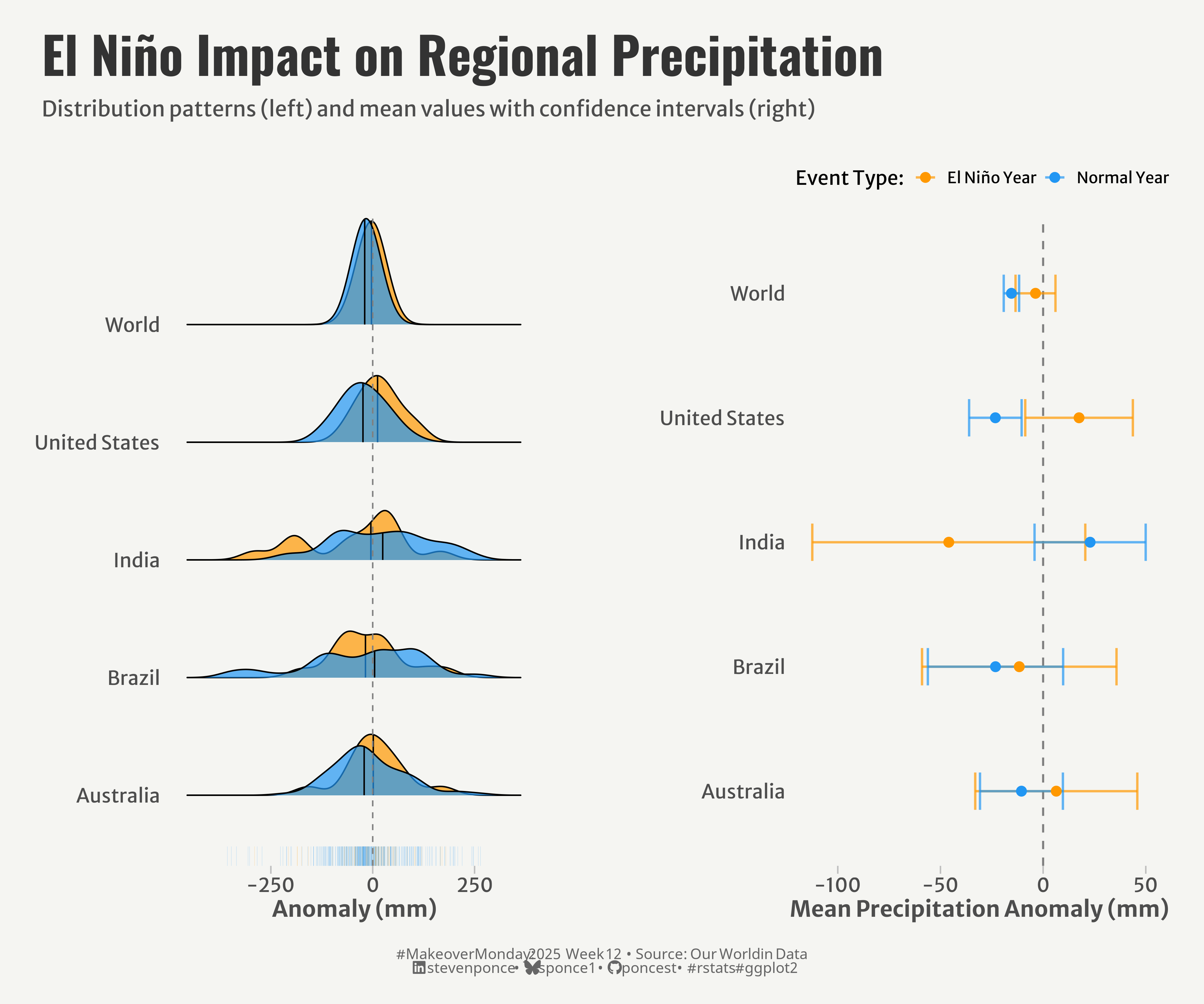
title: "El Niño Impact on Regional Precipitation"
subtitle: "Distribution patterns and mean values with confidence intervals"
description: "Analysis of precipitation anomalies during El Niño events compared to normal years across five global regions. This visualization reveals how El Niño Southern Oscillation affects rainfall patterns differently around the world, using complementary statistical approaches to show both distribution patterns and statistical significance."
author: "Steven Ponce"
date: "2025-03-18"
categories: ["MakeoverMonday", "2025"]
tags: [
"El Niño", "ENSO", "climate", "precipitation", "ridge plots", "confidence intervals", "statistical visualization", "ggplot2", "patchwork", "ggridges", "weather patterns", "climate analysis"
]
image: "thumbnails/mm_2025_12.png"
format:
html:
toc: true
toc-depth: 5
code-link: true
code-fold: true
code-tools: true
code-summary: "Show code"
editor_options:
chunk_output_type: inline
execute:
freeze: true
cache: true
error: false
message: false
warning: false
eval: true
# filters:
# - social-share
# share:
# permalink: "https://stevenponce.netlify.app/data_visualizations/MakeoverMonday/2025/mm_2025_12.html"
# description: "How El Niño affects rainfall across different regions: density patterns and statistical analysis reveal complex precipitation changes beyond simple averages #DataViz #MakeoverMonday #ClimateData"
# twitter: true
# linkedin: true
# email: true
# facebook: false
# reddit: false
# stumble: false
# tumblr: false
# mastodon: true
# bsky: true
---
### Original
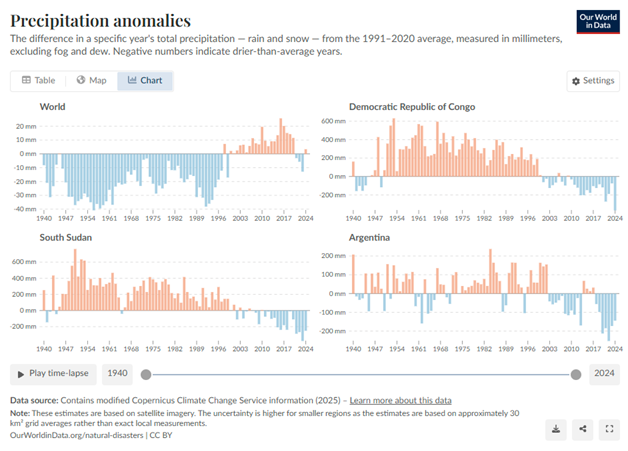
The original visualization __Precipitation Anomalies__ comes from [Our World in Data](https://ourworldindata.org/grapher/global-precipitation-anomaly)
### Makeover
{#fig-1}
### <mark> **Steps to Create this Graphic** </mark>
#### 1. Load Packages & Setup
```{r}
#| label: load
#| warning: false
#| message: false
#| results: "hide"
## 1. LOAD PACKAGES & SETUP ----
suppressPackageStartupMessages({
  if (!require("pacman")) install.packages("pacman")
  pacman::p_load(
      tidyverse,      # Easily Install and Load the 'Tidyverse'
    ggtext,         # Improved Text Rendering Support for 'ggplot2'
    showtext,       # Using Fonts More Easily in R Graphs
    janitor,        # Simple Tools for Examining and Cleaning Dirty Data
    skimr,          # Compact and Flexible Summaries of Data
    scales,         # Scale Functions for Visualization
    glue,           # Interpreted String Literals
    here,           # A Simpler Way to Find Your Files
    lubridate,      # Make Dealing with Dates a Little Easier
    ggridges,       # Ridgeline Plots in 'ggplot2' # Ridgeline Plots in 'ggplot2'
    patchwork,      # The Composer of Plots
    camcorder       # Record Your Plot History
  )
})

### |- figure size ----
gg_record(
    dir    = here::here("temp_plots"),
    device = "png",
    width  =  12,
    height =  10,
    units  = "in",
    dpi    = 320
)

# Source utility functions
suppressMessages(source(here::here("R/utils/fonts.R")))
source(here::here("R/utils/social_icons.R"))
source(here::here("R/utils/image_utils.R"))
source(here::here("R/themes/base_theme.R"))
```
#### 2. Read in the Data
```{r}
#| label: read
#| include: true
#| eval: true
#| warning: false
#' The raw data for the week MakeoverMonday challenge can be downloaded
#' https://data.world/makeovermonday/2025w12-precipitation-anomalies
#'
#' Article
#' https://ourworldindata.org/grapher/global-precipitation-anomaly

precipitation_raw <- read_csv(
  here::here('data/global-precipitation-anomaly.csv')) |>
    clean_names()
```
#### 3. Examine the Data
```{r}
#| label: examine
#| include: true
#| eval: true
#| results: 'hide'
#| warning: false
glimpse(precipitation_raw)
skim(precipitation_raw)
```
#### 4. Tidy Data
```{r}
#| label: tidy
#| warning: false
### |-  tidy data ----
# Define El Niño years based on moderate to strong events
el_nino_years <- c(1982, 1983, 1987, 1988, 1991, 1992, 1997, 1998,
                   2002, 2003, 2009, 2010, 2015, 2016)

# ENSO (El Niño Southern Oscillation) data
enso_data <- precipitation_raw |>
  filter(entity %in% c('World', 'Brazil', 'Australia', 'India', 'United States')) |>
  mutate(
    el_nino = year %in% el_nino_years,
    event_type = if_else(el_nino, 'El Niño Year', 'Normal Year')
  )

# Comparative statistics for El Niño vs Normal
comparative_stats <- enso_data |>
  group_by(entity, event_type) |>
  summarize(
    mean_anomaly = mean(annual_precipitation_anomaly, na.rm = TRUE),
    median_anomaly = median(annual_precipitation_anomaly, na.rm = TRUE),
    sd_anomaly = sd(annual_precipitation_anomaly, na.rm = TRUE),
    n_obs = n(),
    se_anomaly = sd_anomaly / sqrt(n_obs),
    ci_lower = mean_anomaly - 1.96 * se_anomaly,
    ci_upper = mean_anomaly + 1.96 * se_anomaly,
    .groups = 'drop'
  )
```
#### 5. Visualization Parameters
```{r}
#| label: params
#| include: true
#| warning: false
### |-  plot aesthetics ----
# Get base colors with custom palette
colors <- get_theme_colors(palette = c(
  'El Niño Year' = '#FF9800',
  'Normal Year' = '#2196F3'
))

### |-  titles and caption ----
title_text <- str_glue("El Niño Impact on Regional Precipitation")
subtitle_text <- str_glue("Distribution patterns (left) and mean values with confidence intervals (right)")

# Create caption
caption_text <- create_mm_caption(
    mm_year = 2025,
    mm_week = 12,
    source_text = "Our World in Data"
)

### |-  fonts ----
setup_fonts()
fonts <- get_font_families()

### |-  plot theme ----

# Start with base theme
base_theme <- create_base_theme(colors)

# Add weekly-specific theme elements
weekly_theme <- extend_weekly_theme(
  base_theme,
  theme(
    # Weekly-specific modifications
    legend.position = "plot",

    axis.title = element_text(size = rel(1.14)),
    axis.text = element_text(size = rel(1)),

    axis.ticks.y = element_blank(),
    axis.ticks.x = element_line(color = "gray", linewidth = 0.5),
    axis.ticks.length = unit(0.2, "cm"),

    panel.border = element_blank(),
    panel.grid = element_blank(),
    panel.spacing = unit(1, "lines"),
    panel.spacing.y = unit(0, "lines"),

  )
)

# Set theme
theme_set(weekly_theme)
```
#### 6. Plot
```{r}
#| label: plot
#| warning: false
### |-  Plot  ----
# P1. Ridges Chart ----
p1 <- ggplot(enso_data, aes(x = annual_precipitation_anomaly, y = entity, fill = event_type)) +
  # Geoms
  geom_density_ridges(
    scale = 0.9,
    alpha = 0.7,
    quantile_lines = TRUE,
    quantiles = c(0.5),
    jittered_points = FALSE
  ) +
  geom_rug(
    aes(color = event_type),
    alpha = 0.3,
    size = 0.1,
    sides = "b",
    position = position_nudge(y = -0.2)
  ) +
  geom_vline(xintercept = 0, linetype = "dashed", color = "gray50") +
  # Scales
  scale_x_continuous() +
  scale_y_discrete() +
  scale_fill_manual(values = colors$palette) +
  scale_color_manual(values = colors$palette) +
  coord_cartesian(clip = 'off') +
  # Labs
  labs(
    x = 'Anomaly (mm)',
    y = NULL,
    fill = 'Year Type',
  )

# P2. Dot Plot ----
p2 <-ggplot(comparative_stats, aes(x = mean_anomaly, y = entity, color = event_type)) +
  # Geoms
  geom_vline(xintercept = 0, linetype = "dashed", color = "gray50", size = 0.7) +
  geom_errorbarh(
    aes(xmin = ci_lower, xmax = ci_upper),
    height = 0.3,
    size = 0.8,
    alpha = 0.7
  ) +
  geom_point(size = 3) +
  # Scales
  scale_x_continuous() +
  scale_y_discrete() +
  scale_color_manual(
    values = colors$palette
  ) +
  coord_cartesian(clip = 'off') +
  # Labs
  labs(
    x = "Mean Precipitation Anomaly (mm)",
    y = NULL,
    color = "Event Type: "
  ) +
  # Theme
  theme(legend.position = "top")

# Combined Plots ----
combined_plot <- (p1 | plot_spacer() | p2) +
  plot_layout(
    widths = c(1, 0.05, 1),
    nrow = 1) +
  plot_annotation(
    title = title_text,
    subtitle = subtitle_text,
    caption = caption_text,
    theme = theme(
      plot.title = element_text(
        size   = rel(2.6),
        family = fonts$title,
        face   = "bold",
        color  = colors$title,
        lineheight = 1.1,
        margin = margin(t = 5, b = 5)
      ),
      plot.subtitle = element_text(
        size   = rel(1.1),
        family = fonts$subtitle,
        color  = colors$subtitle,
        lineheight = 1.2,
        margin = margin(t = 5, b = 15)
      ),
      plot.caption = element_markdown(
        size   = rel(0.75),
        family = fonts$caption,
        color  = colors$caption,
        hjust  = 0.5,
        margin = margin(t = 10)
      ),
      plot.margin = margin(t = 20, r = 10, b = 20, l = 10)
      )
    )
```
#### 7. Save
```{r}
#| label: save
#| warning: false
### |-  plot image ----
save_plot_patchwork(
  combined_plot,
  type = "makeovermonday",
  year = 2025,
  week = 12,
  width = 12,
  height = 10
  )
```
#### 8. Session Info
::: {.callout-tip collapse="true"}
##### Expand for Session Info
```{r, echo = FALSE}
#| eval: true
#| warning: false
sessionInfo()
```
:::
#### 9. GitHub Repository
::: {.callout-tip collapse="true"}
##### Expand for GitHub Repo
The complete code for this analysis is available in [`mm_2025_12.qmd`](https://github.com/poncest/personal-website/blob/master/data_visualizations/MakeoverMonday/2025/mm_2025_12.qmd).
For the full repository, [click here](https://github.com/poncest/personal-website/).
:::
#### 10. References
::: {.callout-tip collapse="true"}
##### Expand for References
1. Data:
- Makeover Monday 2025 Week 12: [Precipitation anomalies](https://data.world/makeovermonday/2025w12-precipitation-anomalies)
2. Article
- Precipitation anomalies: [Precipitation anomalies](https://ourworldindata.org/grapher/global-precipitation-anomaly)
:::

