---
title: "London Underground Temperature Analysis (2013-2023)"
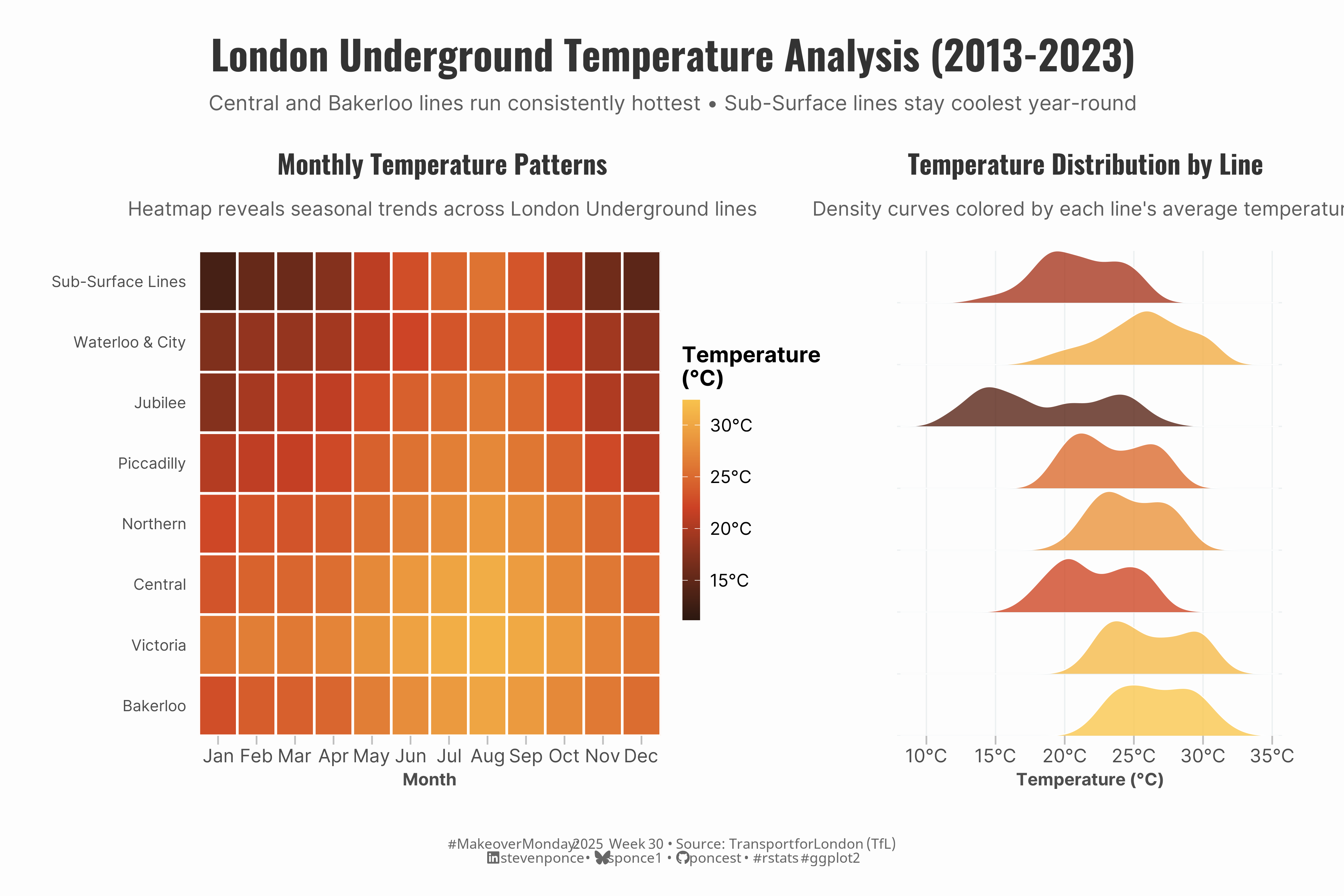
subtitle: "Central and Bakerloo lines run consistently hottest • Sub-Surface lines stay coolest year-round"
description: "A MakeoverMonday data visualization analyzing 10 years of London Underground temperature data. Using unified warm color palettes, this dual-chart approach reveals how Central and Bakerloo lines consistently run 5-10°C hotter than Sub-Surface lines, with summer creating the starkest temperature differences across the network."
author: "Steven Ponce"
date: "2025-07-23"
categories: ["MakeoverMonday", "2025"]
tags: [
"london-underground",
"temperature-analysis",
"heatmap",
"ridgeline-plot",
"ggplot2",
"ggridges",
"patchwork",
"warm-colors",
"public-transport",
"seasonal-patterns",
"tfl-data",
"unified-color-palette",
"horizontal-scanning",
"data-storytelling"
]
image: "thumbnails/mm_2025_30.png"
format:
html:
toc: true
toc-depth: 5
code-link: true
code-fold: true
code-tools: true
code-summary: "Show code"
editor_options:
chunk_output_type: inline
execute:
freeze: true
cache: true
error: false
message: false
warning: false
eval: true
---
```{r}
#| label: setup-links
#| include: false
# CENTRALIZED LINK MANAGEMENT
## Project-specific info
current_year <- 2025
current_week <- 30
project_file <- "mm_2025_30.qmd"
project_image <- "mm_2025_30.png"
## Data Sources
data_main <- "https://data.world/makeovermonday/2025w30-london-underground-average-monthly-temperatures/settings?tab=access"
data_secondary <- "https://www.dailymail.co.uk/sciencetech/article-13739705/london-underground-hottest-line.html"
## Repository Links
repo_main <- "https://github.com/poncest/personal-website/"
repo_file <- paste0("https://github.com/poncest/personal-website/blob/master/data_visualizations/MakeoverMonday/", current_year, "/", project_file)
## External Resources/Images
chart_original <- "https://raw.githubusercontent.com/poncest/MakeoverMonday/refs/heads/master/2025/Week_30/original_chart.png"
## Organization/Platform Links
org_primary <- "https://data.london.gov.uk/dataset/london-underground-average-monthly-temperatures/"
org_secondary <- "https://data.world/makeovermonday"
# Helper function to create markdown links
create_link <- function(text, url) {
paste0("[", text, "](", url, ")")
}
# Helper function for citation-style links
create_citation_link <- function(text, url, title = NULL) {
if (is.null(title)) {
paste0("[", text, "](", url, ")")
} else {
paste0("[", text, "](", url, ' "', title, '")')
}
}
```
### Original
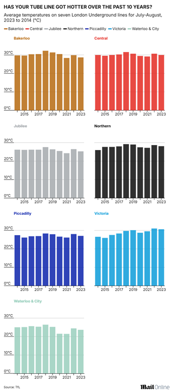
The original visualization **HAS YOUR TUBE LINE GOT HOTTER OVER THE PAST 10 YEARS? Average temperatures on seven London Underground lines for July-August, 2023 to 2014 (°C)** comes from `r create_link("Transport for London (TfL)", data_secondary)`

### Makeover
{#fig-1}
### <mark> **Steps to Create this Graphic** </mark>
#### 1. Load Packages & Setup
```{r}
#| label: load
#| warning: false
#| message: false
#| results: "hide"

## 1. LOAD PACKAGES & SETUP ----
suppressPackageStartupMessages({
  if (!require("pacman")) install.packages("pacman")
  pacman::p_load(
  tidyverse,      # Easily Install and Load the 'Tidyverse'
  ggtext,         # Improved Text Rendering Support for 'ggplot2'
  showtext,       # Using Fonts More Easily in R Graphs
  scales,         # Scale Functions for Visualization
  glue,           # Interpreted String Literals
  patchwork,      # The Composer of Plots
  ggridges        # Ridgeline Plots in 'ggplot2'
  )
})

### |- figure size ----
camcorder::gg_record(
    dir    = here::here("temp_plots"),
    device = "png",
    width  =  12,
    height =  8,
    units  = "in",
    dpi    = 320
)

# Source utility functions
suppressMessages(source(here::here("R/utils/fonts.R")))
source(here::here("R/utils/social_icons.R"))
source(here::here("R/utils/image_utils.R"))
source(here::here("R/themes/base_theme.R"))
```
#### 2. Read in the Data
```{r}
#| label: read
#| include: true
#| eval: true
#| warning: false
#|
avg_temp_raw <- read_csv(
  here::here('data/MakeoverMonday/2025/lu-average-monthly-temperatures 2013-2024.csv')) |>
  janitor::clean_names()
```
#### 3. Examine the Data
```{r}
#| label: examine
#| include: true
#| eval: true
#| results: 'hide'
#| warning: false

glimpse(avg_temp_raw)
skimr::skim(avg_temp_raw)
```
#### 4. Tidy Data
```{r}
#| label: tidy
#| warning: false

temp_long <- avg_temp_raw |>
  pivot_longer(cols = bakerloo:sub_surface_lines,
               names_to = "line",
               values_to = "temperature") |>
  mutate(
    date = ymd(paste(year, month, "01")),
    month_num = match(month, month.name),
    season = case_when(
      month_num %in% c(12, 1, 2) ~ "Winter",
      month_num %in% c(3, 4, 5) ~ "Spring",
      month_num %in% c(6, 7, 8) ~ "Summer",
      month_num %in% c(9, 10, 11) ~ "Autumn"
    ),
    line_clean = case_when(
      line == "waterloo_and_city" ~ "Waterloo & City",
      line == "sub_surface_lines" ~ "Sub-Surface Lines",
      TRUE ~ str_to_title(line)
    )
  )

line_order <- temp_long |>
  group_by(line_clean) |>
  summarise(median_temp = median(temperature, na.rm = TRUE), .groups = "drop") |>
  arrange(desc(median_temp)) |>
  pull(line_clean)
```
#### 5. Visualization Parameters
```{r}
#| label: params
#| include: true
#| warning: false

### |-  plot aesthetics ----
# Get base colors with custom palette
colors <- get_theme_colors(palette = list(NULL))

### |-  titles and caption ----
title_text <- str_glue("London Underground Temperature Analysis (2013-2023)")
subtitle_text <- str_glue("Central and Bakerloo lines run consistently hottest • Sub-Surface lines stay coolest year-round")

# Create caption
caption_text <- create_mm_caption(
  mm_year = current_year,
  mm_week = current_week,
  source_text = paste0("Transport for London (TfL)")
)

### |-  fonts ----
setup_fonts()
fonts <- get_font_families()

### |-  plot theme ----

# Start with base theme
base_theme <- create_base_theme(colors)

# Add weekly-specific theme elements
weekly_theme <- extend_weekly_theme(
  base_theme,
  theme(
    plot.title = element_text(
      size = rel(1.2), family = fonts$title, face = "bold",
      color = colors$title, lineheight = 1.1, hjust = 0.5,
      margin = margin(t = 5, b = 10)
    ),
    plot.subtitle = element_text(
      size = rel(0.9), hjust = 0.5, family = fonts$subtitle,
      color = alpha(colors$subtitle, 0.9), lineheight = 0.9,
      margin = margin(t = 5, b = 20)
    ),

    # Legend formatting
    legend.position = "right",
    # legend.direction = "horizontal",
    legend.box.margin = margin(b = 10),
    legend.margin = margin(b = 5),
    legend.title = element_text(face = "bold"),

    # Axis formatting
    axis.ticks.y = element_blank(),
    axis.ticks.x = element_line(color = "gray", linewidth = 0.5),
    axis.ticks.length = unit(0.2, "cm"),
    axis.title.x = element_text(face = "bold", size = rel(0.85)),
    axis.title.y = element_text(face = "bold", size = rel(0.85)),
    axis.text = element_text(size = rel(0.85), family = fonts$subtitle, color = colors$text),

    # Grid lines
    panel.grid.major = element_line(color = "#ecf0f1", linewidth = 0.4),
    panel.grid.minor = element_blank(),

    # Margin
    plot.margin = margin(20, 20, 20, 20)
  )
)

# Set theme
theme_set(weekly_theme)

# Scale function
create_warm_color_scale <- function(legend_position = "right") {
  scale_fill_gradient2(
    name = "Temperature\n(°C)",
    low = "#2c1810",
    mid = "#cc4125",
    high = "#f9c74f",
    midpoint = 22,
    breaks = seq(10, 30, 5),
    labels = paste0(seq(10, 30, 5), "°C"),
    guide = if(legend_position == "none") "none" else guide_colorbar()
  )
}
```
#### 6. Plot
```{r}
#| label: plot
#| warning: false

### |-  Plot 1  heatmap ----
p1 <- temp_long |>
  mutate(line_clean = factor(line_clean, levels = line_order)) |>
  ggplot(aes(x = month_num, y = line_clean, fill = temperature)) +
  # Geoms
  geom_tile(color = "white", linewidth = 0.8) +
  # Scales
  create_warm_color_scale() +
  scale_x_continuous(
    breaks = 1:12,
    labels = month.abb,
    expand = c(0, 0)
  ) +
  scale_y_discrete(expand = c(0, 0)) +
  # Labs
  labs(
    title = "Monthly Temperature Patterns",
    subtitle = "Heatmap reveals seasonal trends across London Underground lines",
    x = "Month",
    y = NULL
  ) +
  # Theme
  theme(
    legend.position = "right",
    legend.key.height = unit(1, "cm"),
    legend.key.width = unit(0.4, "cm"),
    axis.text.y = element_text(size = 10, hjust = 1)
  )

### |-  Plot 2  ridges plot ----
# Calculate average temperature for each line
line_avg_temps <- temp_long |>
  group_by(line_clean) |>
  summarise(avg_temp = mean(temperature, na.rm = TRUE), .groups = "drop")

p2 <- temp_long |>
  mutate(line_clean = factor(line_clean, levels = line_order)) |>
  left_join(line_avg_temps, by = "line_clean") |>
  ggplot(aes(x = temperature, y = line_clean, fill = avg_temp)) +
  # Geoms
  geom_density_ridges(
    alpha = 0.8,
    scale = 0.95,
    linewidth = 0.3,
    color = "white"
  ) +
  # Scales
  create_warm_color_scale(legend_position = "none") +
  scale_x_continuous(
    breaks = seq(10, 35, 5),
    labels = paste0(seq(10, 35, 5), "°C"),
    expand = c(0.01, 0)
  ) +
  scale_y_discrete(expand = c(0, 0)) +
  # Labs
  labs(
    title = "Temperature Distribution by Line",
    subtitle = "Density curves colored by each line's average temperature",
    x = "Temperature (°C)",
    y = NULL
  ) +
  # Theme
  theme(
    axis.text.y = element_blank(),
    axis.ticks.y = element_blank()
  )

### |-  combined plot ----
# Create an invisible spacer plot
spacer <- ggplot() +
  theme_void()

combined_plots <- (p1 + spacer + p2) +
  plot_layout(
    widths = c(1.2, 0.01, 1)
    )

combined_plots <- combined_plots +
  plot_annotation(
    title = title_text,
    subtitle = subtitle_text,
    caption = caption_text,
    theme = theme(
      plot.title = element_text(
        size = rel(1.85),
        family = fonts$title,
        face = "bold",
        hjust = 0.5,
        color = colors$title,
        lineheight = 1.1,
        margin = margin(t = 5, b = 5)
      ),
      plot.subtitle = element_text(
        size = rel(0.95),
        hjust = 0.5,
        family = fonts$subtitle,
        color = alpha(colors$subtitle, 0.9),
        lineheight = 0.9,
        margin = margin(t = 5, b = 0)
      ),
      plot.caption = element_markdown(
        size = rel(0.65),
        family = fonts$caption,
        color = colors$caption,
        hjust = 0.5,
        margin = margin(t = 10)
      )
    )
  )
```
#### 7. Save
```{r}
#| label: save
#| warning: false

### |-  plot image ----
save_plot_patchwork(
  plot = combined_plots,
  type = "makeovermonday",
  year = current_year,
  week = current_week,
  width = 12,
  height = 8
  )
```
#### 8. Session Info
::: {.callout-tip collapse="true"}
##### Expand for Session Info
```{r, echo = FALSE}
#| eval: true
#| warning: false
sessionInfo()
```
:::
#### 9. GitHub Repository
::: {.callout-tip collapse="true"}
##### Expand for GitHub Repo
The complete code for this analysis is available in `r create_link(project_file, repo_file)`.
For the full repository, `r create_link("click here", repo_main)`.
:::
#### 10. References
::: {.callout-tip collapse="true"}
##### Expand for References
1. Data:
- Makeover Monday `r current_year` Week `r current_week`: `r create_link("London Underground Average Monthly Temperatures", data_main)`
2. Article
- `r create_link("Daily Mail Online: Is your commute a scorcher?", data_secondary)`
:::