---
title: "Global Meat Production Analysis: Trends & Statistical Precision"
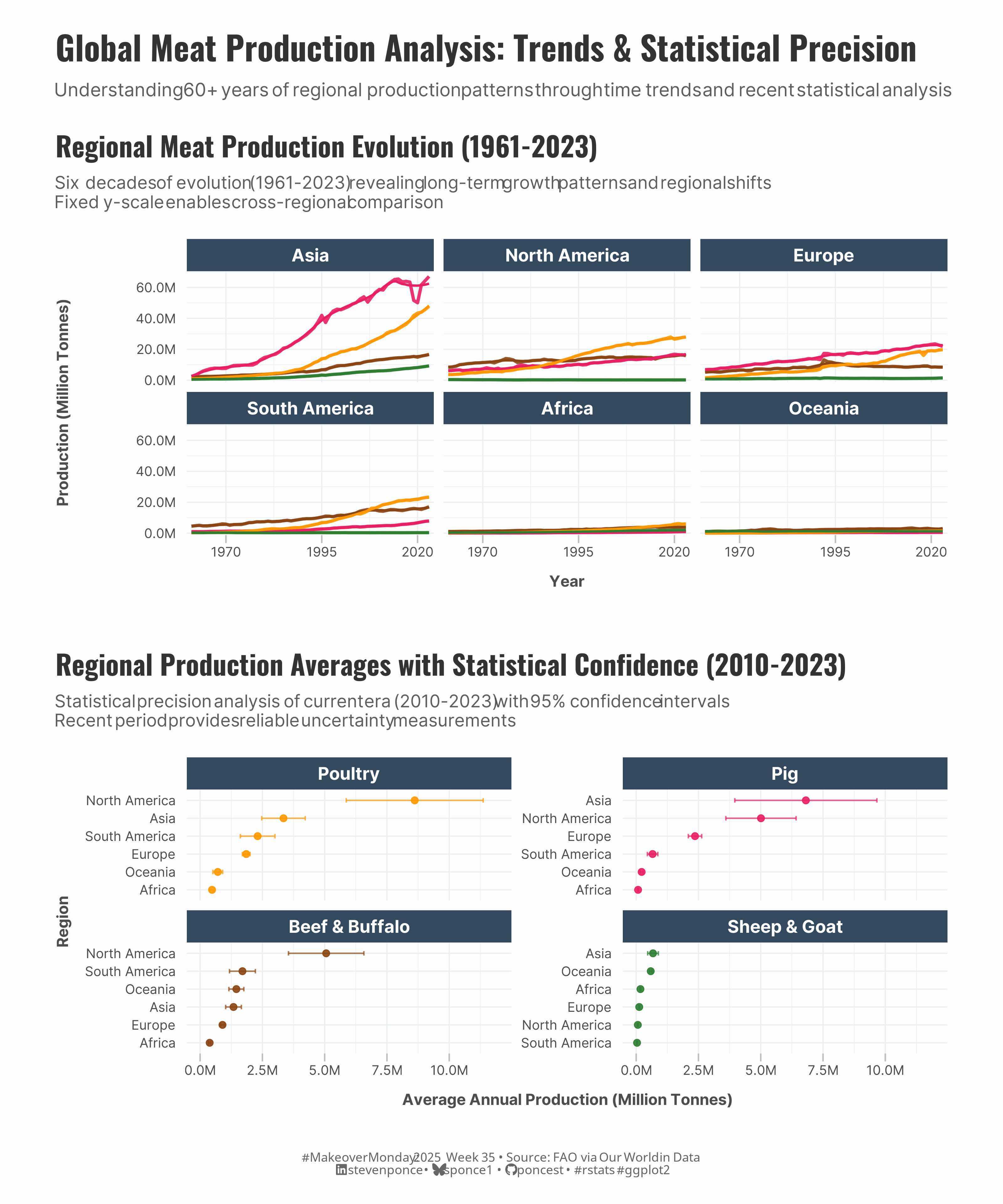
subtitle: "Understanding 60+ years of regional production patterns through time trends and recent statistical analysis"
description: "A comprehensive analysis of global meat production from 1961-2023, combining historical trend visualization with statistical precision analysis. This MakeoverMonday project transforms FAO data into a dual-panel visualization that reveals Asia's dramatic rise in meat production while providing statistical confidence intervals for current production levels across six regions and four major meat types."
author: "Steven Ponce"
date: "2025-08-26"
categories: ["MakeoverMonday", "2025"]
tags: [
"meat production",
"global agriculture",
"time series analysis",
"statistical visualization",
"confidence intervals",
"regional comparison",
"faceted plots",
"food security",
"agricultural trends",
"ggplot2",
"tidytext",
"patchwork"
]
image: "thumbnails/mm_2025_35.png"
format:
html:
toc: true
toc-depth: 5
code-link: true
code-fold: true
code-tools: true
code-summary: "Show code"
editor_options:
chunk_output_type: inline
execute:
freeze: true
cache: true
error: false
message: false
warning: false
eval: true
---
```{r}
#| label: setup-links
#| include: false
# CENTRALIZED LINK MANAGEMENT
## Project-specific info
current_year <- 2025
current_week <- 35
project_file <- "mm_2025_35.qmd"
project_image <- "mm_2025_35.png"
## Data Sources
data_main <- "https://ourworldindata.org/meat-production"
data_secondary <- "https://ourworldindata.org/meat-production"
## Repository Links
repo_main <- "https://github.com/poncest/personal-website/"
repo_file <- paste0("https://github.com/poncest/personal-website/blob/master/data_visualizations/MakeoverMonday/", current_year, "/", project_file)
## External Resources/Images
chart_original <- "https://raw.githubusercontent.com/poncest/MakeoverMonday/refs/heads/master/2025/Week_35/original_chart.png"
## Organization/Platform Links
org_primary <- "https://ourworldindata.org/meat-production"
org_secondary <- "https://ourworldindata.org/"
# Helper function to create markdown links
create_link <- function(text, url) {
paste0("[", text, "](", url, ")")
}
# Helper function for citation-style links
create_citation_link <- function(text, url, title = NULL) {
if (is.null(title)) {
paste0("[", text, "](", url, ")")
} else {
paste0("[", text, "](", url, ' "', title, '")')
}
}
```
### Original
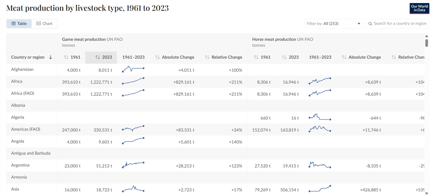
The original visualization **Global meat production, 1961 to 2023** comes from `r create_link("Food and Agriculture Organization of the United Nations (2025)", data_secondary)`
<!--  -->
### Makeover
{#fig-1}
### <mark> **Steps to Create this Graphic** </mark>
#### 1. Load Packages & Setup
```{r}
#| label: load
#| warning: false
#| message: false
#| results: "hide"

## 1. LOAD PACKAGES & SETUP ----
suppressPackageStartupMessages({
  if (!require("pacman")) install.packages("pacman")
  pacman::p_load(
    tidyverse,  # Easily Install and Load the 'Tidyverse'
    ggtext,     # Improved Text Rendering Support for 'ggplot2'
    showtext,   # Using Fonts More Easily in R Graphs
    scales,     # Scale Functions for Visualization
    glue,       # Interpreted String Literals
    patchwork,  # The Composer of Plots
    tidytext    # Text Mining using 'dplyr', 'ggplot2', and Other Tidy Tools
  )
})

### |- figure size ----
camcorder::gg_record(
    dir    = here::here("temp_plots"),
    device = "png",
    width  = 10,
    height = 10,
    units  = "in",
    dpi    = 320
)

# Source utility functions
suppressMessages(source(here::here("R/utils/fonts.R")))
source(here::here("R/utils/social_icons.R"))
source(here::here("R/utils/image_utils.R"))
source(here::here("R/themes/base_theme.R"))
```
#### 2. Read in the Data
```{r}
#| label: read
#| include: true
#| eval: true
#| warning: false
#|
meat_production_raw <- readxl::read_excel(
  here::here('data/MakeoverMonday/2025/Global meat production by livestock type.xlsx')) |>
  janitor::clean_names()
```
#### 3. Examine the Data
```{r}
#| label: examine
#| include: true
#| eval: true
#| results: 'hide'
#| warning: false

glimpse(meat_production_raw)
skimr::skim_without_charts(meat_production_raw)
```
#### 4. Tidy Data
```{r}
#| label: tidy
#| warning: false

meat_clean <- meat_production_raw |>
  filter(!is.na(entity), !entity %in% c("World", "")) |>
  pivot_longer(
    cols = starts_with("meat_"),
    names_to = "meat_type_raw",
    values_to = "production_tonnes",
    values_drop_na = TRUE
  ) |>
  # Clean meat type names
  mutate(
    meat_type = case_when(
      str_detect(meat_type_raw, "beef") ~ "Beef & Buffalo",
      str_detect(meat_type_raw, "pig") ~ "Pig",
      str_detect(meat_type_raw, "poultry") ~ "Poultry",
      str_detect(meat_type_raw, "sheep") ~ "Sheep & Goat",
      str_detect(meat_type_raw, "game") ~ "Game",
      str_detect(meat_type_raw, "horse") ~ "Horse",
      str_detect(meat_type_raw, "camel") ~ "Camel",
      TRUE ~ "Other"
    )
  ) |>
  # Focus on major meat types for cleaner visualizations
  filter(meat_type %in% c("Beef & Buffalo", "Pig", "Poultry", "Sheep & Goat")) |>
  select(entity, code, year, meat_type, production_tonnes)

# Create regional groupings for continental analysis
regional_data <- meat_clean |>
  mutate(
    region = case_when(
      entity %in% c(
        "China", "India", "Japan", "South Korea", "Indonesia", "Thailand",
        "Philippines", "Vietnam", "Malaysia", "Bangladesh", "Pakistan"
      ) ~ "Asia",
      entity %in% c("United States", "Canada", "Mexico") ~ "North America",
      entity %in% c(
        "Brazil", "Argentina", "Chile", "Colombia", "Peru", "Uruguay",
        "Venezuela", "Ecuador", "Bolivia"
      ) ~ "South America",
      entity %in% c(
        "Germany", "France", "United Kingdom", "Italy", "Spain", "Poland",
        "Netherlands", "Russia", "Ukraine", "Turkey"
      ) ~ "Europe",
      entity %in% c(
        "Nigeria", "Ethiopia", "South Africa", "Kenya", "Ghana", "Morocco",
        "Algeria", "Egypt", "Tanzania", "Uganda"
      ) ~ "Africa",
      entity %in% c("Australia", "New Zealand") ~ "Oceania",
      TRUE ~ "Other"
    )
  ) |>
  filter(region != "Other")

# P1: Regional trends over time data ----
trends_data <- regional_data |>
  group_by(region, year, meat_type) |>
  summarise(total_production = sum(production_tonnes, na.rm = TRUE), .groups = "drop") |>
  # Calculate growth rates
  group_by(region, meat_type) |>
  arrange(year) |>
  mutate(
    growth_from_start = (total_production / first(total_production) - 1) * 100
  ) |>
  ungroup() |>
  # Order regions by total 2023 production
  group_by(region) |>
  mutate(region_total_2023 = sum(total_production[year == 2023], na.rm = TRUE)) |>
  ungroup() |>
  mutate(region = fct_reorder(region, desc(region_total_2023)))

# P2: Statistical precision data ----
precision_data <- regional_data |>
  filter(year >= 2010) |>
  group_by(region, meat_type) |>
  summarise(
    n_years = n(),
    mean_production = mean(production_tonnes, na.rm = TRUE),
    sd_production = sd(production_tonnes, na.rm = TRUE),
    se_production = sd_production / sqrt(n_years),
    .groups = "drop"
  ) |>
  mutate(
    # 95% confidence intervals
    lower_ci = pmax(0, mean_production - 1.96 * se_production),
    upper_ci = mean_production + 1.96 * se_production
  ) |>
  # Order meat types by total global production
  group_by(meat_type) |>
  mutate(meat_total = sum(mean_production)) |>
  ungroup() |>
  mutate(meat_type_ordered = fct_reorder(meat_type, desc(meat_total))) |>
  # Use tidytext::reorder_within for proper within-facet ordering
  mutate(region_ordered = reorder_within(region, mean_production, meat_type_ordered))
```
#### 5. Visualization Parameters
```{r}
#| label: params
#| include: true
#| warning: false

### |-  plot aesthetics ----
# Get base colors with custom palette
colors <- get_theme_colors(palette = c(
  "Beef & Buffalo" = "#8B4513",
  "Pig" = "#E91E63",
  "Poultry" = "#FF9800",
  "Sheep & Goat" = "#2E7D32"
))

### |-  titles and caption ----
title_text <- str_glue("Global Meat Production Analysis: Trends & Statistical Precision")

subtitle_text <- str_glue(
  "Understanding 60+ years of regional production patterns through time trends and recent statistical analysis"
)

# Create caption
caption_text <- create_mm_caption(
  mm_year = current_year,
  mm_week = current_week,
  source_text = paste0("FAO via Our World in Data")
)

### |-  fonts ----
setup_fonts()
fonts <- get_font_families()

### |-  plot theme ----

# Start with base theme
base_theme <- create_base_theme(colors)

# Add weekly-specific theme elements
weekly_theme <- extend_weekly_theme(
  base_theme,
  theme(
    plot.title = element_text(
      size = rel(1.4), family = fonts$title, face = "bold",
      color = colors$title, lineheight = 1.1, hjust = 0,
      margin = margin(t = 5, b = 10)
    ),
    plot.subtitle = element_markdown(
      size = rel(0.9), family = fonts$subtitle, face = "italic",
      color = alpha(colors$subtitle, 0.9), lineheight = 1.1,
      margin = margin(t = 0, b = 20)
    ),

    # Legend formatting
    legend.position = "plot",
    legend.justification = "top",
    legend.margin = margin(l = 12, b = 5),
    legend.key.size = unit(0.8, "cm"),
    legend.box.margin = margin(b = 10),
    legend.title = element_text(face = "bold"),

    # Axis formatting
    axis.ticks.y = element_blank(),
    axis.ticks.x = element_line(color = "gray", linewidth = 0.5),
    axis.ticks.length = unit(0.2, "cm"),
    axis.title.x = element_text(
      face = "bold", size = rel(0.85),
      margin = margin(t = 10)
    ),
    axis.title.y = element_text(
      face = "bold", size = rel(0.85),
      margin = margin(r = 10)
    ),
    axis.text.x = element_text(
      size = rel(0.85), family = fonts$subtitle,
      color = colors$text
    ),
    axis.text.y = element_text(
      size = rel(0.85), family = fonts$subtitle,
      color = colors$text
    ),

    # Grid lines
    panel.grid.minor = element_line(color = "#ecf0f1", linewidth = 0.2),
    panel.grid.major = element_line(color = "#ecf0f1", linewidth = 0.4),

    # Margin
    plot.margin = margin(20, 20, 20, 20)
  )
)

# Set theme
theme_set(weekly_theme)
```
#### 6. Plot
```{r}
#| label: plot
#| warning: false

### |- P1  Regional trends over time chart ----
p1 <- trends_data |>
  ggplot(aes(x = year, y = total_production, color = meat_type)) +

  # Geoms
  geom_line(size = 1.1, alpha = 0.9) +
  geom_smooth(method = "loess", se = FALSE, size = 0.8, alpha = 0.6, span = 0.3) +
  # Scales
  scale_color_manual(values = colors$palette, name = "Meat Type") +
  scale_y_continuous(
    labels = label_number(scale = 1e-6, suffix = "M", accuracy = 0.1),
    expand = expansion(mult = c(0.02, 0.05))
  ) +
  scale_x_continuous(
    breaks = seq(1970, 2020, 25),
    expand = expansion(mult = c(0.02, 0.02))
  ) +
  # Labs
  labs(
    title = "Regional Meat Production Evolution (1961-2023)",
    subtitle = str_glue(
      "Six decades of evolution (1961-2023) revealing long-term growth patterns and regional shifts<br>",
      "Fixed y-scale enables cross-regional comparison"
    ),
    x = "Year",
    y = "Production (Million Tonnes)"
  ) +
  # Facets
  facet_wrap(~region, scales = "fixed", ncol = 3) +
  # Theme
  theme(
    strip.text = element_text(face = "bold", size = rel(0.9), color = "white", family = fonts$text),
    strip.background = element_rect(fill = "#34495e", color = NA),
    )

### |- P2  Statistical precision chart----
p2 <- precision_data |>
  ggplot(aes(x = mean_production, y = region_ordered, color = meat_type)) +
  # Geoms
  geom_errorbarh(
    aes(xmin = lower_ci, xmax = upper_ci),
    height = 0.25, alpha = 0.7, linewidth = 0.5
  ) +
  geom_point(size = 2, alpha = 0.9) +
  # Scales
  scale_color_manual(values = colors$palette, guide = "none") +
  scale_x_continuous(
    labels = label_number(scale = 1e-6, suffix = "M", accuracy = 0.1),
    expand = expansion(mult = c(0.05, 0.1))
  ) +
  scale_y_reordered() +
  # Labs
  labs(
    title = "Regional Production Averages with Statistical Confidence (2010-2023)",
    subtitle = str_glue(
      "Statistical precision analysis of current era (2010-2023) with 95% confidence intervals<br>",
      "Recent period provides reliable uncertainty measurements"
    ),
    x = "Average Annual Production (Million Tonnes)",
    y = "Region"
  ) +
  # Facets
  facet_wrap(~meat_type_ordered, scales = "free_y", ncol = 2) +
  # Theme
  theme(
    strip.text = element_text(face = "bold", size = rel(0.9), color = "white", family = fonts$text),
    strip.background = element_rect(fill = "#34495e", color = NA)
    )

### |-  combined plot ----
combined_plots <- p1 / p2 +
  plot_layout(heights = c(1, 1))

combined_plots <- combined_plots +
  plot_annotation(
    title = title_text,
    subtitle = subtitle_text,
    caption = caption_text,
    theme = theme(
      plot.title = element_text(
        size = rel(1.7),
        family = fonts$title,
        face = "bold",
        color = colors$title,
        lineheight = 1.1,
        margin = margin(t = 5, b = 5)
      ),
      plot.subtitle = element_markdown(
        size = rel(0.95),
        family = fonts$subtitle,
        color = alpha(colors$subtitle, 0.9),
        lineheight = 0.9,
        margin = margin(t = 5, b = 0)
      ),
      plot.caption = element_markdown(
        size = rel(0.65),
        family = fonts$caption,
        color = colors$caption,
        hjust = 0.5,
        margin = margin(t = 10)
      )
    )
  )
```
#### 7. Save
```{r}
#| label: save
#| warning: false

### |-  plot image ----
save_plot_patchwork(
  plot = combined_plots,
  type = "makeovermonday",
  year = current_year,
  week = current_week,
  width = 10,
  height = 12
  )
```
#### 8. Session Info
::: {.callout-tip collapse="true"}
##### Expand for Session Info
```{r, echo = FALSE}
#| eval: true
#| warning: false
sessionInfo()
```
:::
#### 9. GitHub Repository
::: {.callout-tip collapse="true"}
##### Expand for GitHub Repo
The complete code for this analysis is available in `r create_link(project_file, repo_file)`.
For the full repository, `r create_link("click here", repo_main)`.
:::
#### 10. References
::: {.callout-tip collapse="true"}
##### Expand for References
1. Data:
- Makeover Monday `r current_year` Week `r current_week`: `r create_link("Meat Production by Livestock Type", data_main)`
2. Article
- `r create_link("Meat Production by Livestock Type", data_secondary)`
:::

