---
title: "Ranking Drug Harms in the UK"
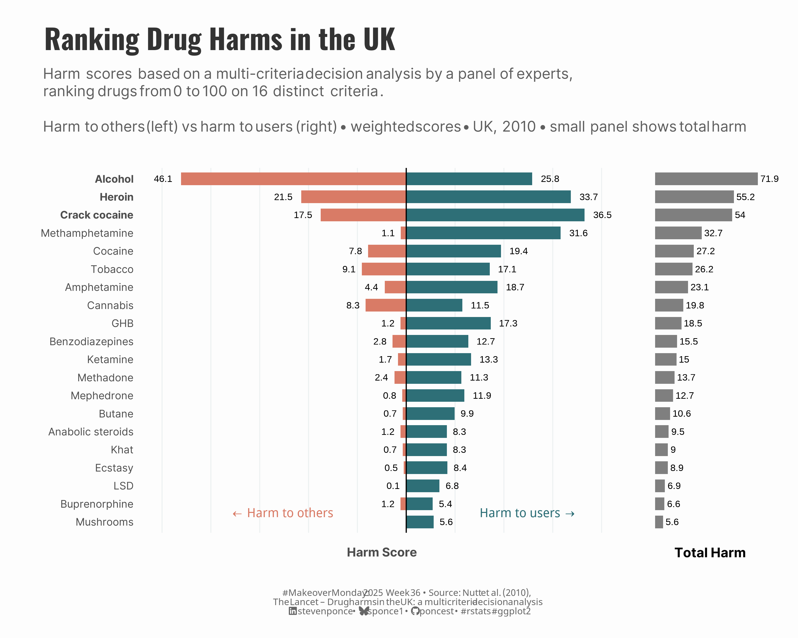
subtitle: "Harm to others vs harm to users • weighted scores • UK, 2010 • small panel shows total harm"
description: "Analysis of the groundbreaking 2010 Lancet study that challenged conventional drug policy by ranking 20 drugs based on evidence rather than legal status. Using multicriteria decision analysis across 16 harm factors, researchers found alcohol causes the most overall harm despite being legal, while many criminalized substances show relatively low harm scores."
date: "2025-09-02"
categories: ["MakeoverMonday", "2025"]
tags: [
"drug policy", "public health", "evidence-based policy", "diverging bars", "Lancet study", "MCDA", "harm reduction", "alcohol harm", "David Nutt", "UK drug classification", "social harm", "individual harm", "policy disconnect", "scientific evidence", "health visualization"
]
image: "thumbnails/mm_2025_36.png"
format:
html:
toc: true
toc-depth: 5
code-link: true
code-fold: true
code-tools: true
code-summary: "Show code"
editor_options:
chunk_output_type: inline
execute:
freeze: true
cache: true
error: false
message: false
warning: false
eval: true
---
```{r}
#| label: setup-links
#| include: false
# CENTRALIZED LINK MANAGEMENT
## Project-specific info
current_year <- 2025
current_week <- 36
project_file <- "mm_2025_36.qmd"
project_image <- "mm_2025_36.png"
## Data Sources
data_main <- "https://data.world/makeovermonday/2025w36-drug-harms-in-the-uk"
data_secondary <- "https://data.world/makeovermonday/2025w36-drug-harms-in-the-uk"
## Repository Links
repo_main <- "https://github.com/poncest/personal-website/"
repo_file <- paste0("https://github.com/poncest/personal-website/blob/master/data_visualizations/MakeoverMonday/", current_year, "/", project_file)
## External Resources/Images
chart_original <- "https://raw.githubusercontent.com/poncest/MakeoverMonday/refs/heads/master/2025/Week_36/original_chart.png"
## Organization/Platform Links
org_primary <- "https://www.economist.com/graphic-detail/2019/06/25/what-is-the-most-dangerous-drug"
org_secondary <- "https://www.economist.com/"
# Helper function to create markdown links
create_link <- function(text, url) {
paste0("[", text, "](", url, ")")
}
# Helper function for citation-style links
create_citation_link <- function(text, url, title = NULL) {
if (is.null(title)) {
paste0("[", text, "](", url, ")")
} else {
paste0("[", text, "](", url, ' "', title, '")')
}
}
```
### Original
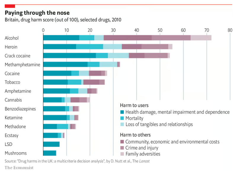
The original visualization **Global meat production, 1961 to 2023** comes from `r create_link("Food and Agriculture Organization of the United Nations (2025)", data_secondary)`
<!--  -->
### Makeover
{#fig-1}
### <mark> **Steps to Create this Graphic** </mark>
#### 1. Load Packages & Setup
```{r}
#| label: load
#| warning: false
#| message: false
#| results: "hide"

## 1. LOAD PACKAGES & SETUP ----
suppressPackageStartupMessages({
  if (!require("pacman")) install.packages("pacman")
  pacman::p_load(
  tidyverse,  # Easily Install and Load the 'Tidyverse'
  ggtext,     # Improved Text Rendering Support for 'ggplot2'
  showtext,   # Using Fonts More Easily in R Graphs
  scales,     # Scale Functions for Visualization
  glue,       # Interpreted String Literals
  patchwork   # The Composer of Plots
  )
})

### |- figure size ----
camcorder::gg_record(
    dir    = here::here("temp_plots"),
    device = "png",
    width  = 10,
    height = 8,
    units  = "in",
    dpi    = 320
)

# Source utility functions
suppressMessages(source(here::here("R/utils/fonts.R")))
source(here::here("R/utils/social_icons.R"))
source(here::here("R/utils/image_utils.R"))
source(here::here("R/themes/base_theme.R"))
```
#### 2. Read in the Data
```{r}
#| label: read
#| include: true
#| eval: true
#| warning: false
#|
drug_harm_raw <- read_csv(
  here::here('data/MakeoverMonday/2025/Drug Harm MCDA - drug_harms_mcda.csv')) |>
  janitor::clean_names()
```
#### 3. Examine the Data
```{r}
#| label: examine
#| include: true
#| eval: true
#| results: 'hide'
#| warning: false

glimpse(drug_harm_raw)
skimr::skim_without_charts(drug_harm_raw)
```
#### 4. Tidy Data
```{r}
#| label: tidy
#| warning: false

drug_totals_actual <- drug_harm_raw |>
  filter(group %in% c("Harm to users", "Harm to others")) |>
  select(-c(category, criteria)) |>
  pivot_longer(cols = -group, names_to = "drug", values_to = "harm_score") |>
  group_by(drug, group) |>
  summarise(harm = sum(harm_score, na.rm = TRUE), .groups = "drop") |>
  pivot_wider(names_from = group, values_from = harm) |>
  janitor::clean_names() |>
  mutate(total_harm = harm_to_users + harm_to_others) |>
  arrange(desc(total_harm))

# Prepare data for diverging bars
diverging_data <- drug_totals_actual |>
  mutate(
    drug_clean = case_when(
      drug == "crack" ~ "Crack cocaine",
      drug == "methylamphet" ~ "Methamphetamine",
      drug == "ghb" ~ "GHB",
      drug == "anabolic_steroids" ~ "Anabolic steroids",
      drug == "lsd" ~ "LSD",
      TRUE ~ str_to_title(drug)
    ),
    harm_to_others_neg = -harm_to_others,
    drug_clean = fct_reorder(drug_clean, total_harm)
  ) |>
  select(drug_clean, harm_to_users, harm_to_others_neg) |>
  pivot_longer(
    cols = c(harm_to_users, harm_to_others_neg),
    names_to = "harm_type", values_to = "harm_value"
  ) |>
  mutate(
    harm_type = case_when(
      harm_type == "harm_to_users" ~ "Harm to users",
      harm_type == "harm_to_others_neg" ~ "Harm to others"
    )
  )
```
#### 5. Visualization Parameters
```{r}
#| label: params
#| include: true
#| warning: false

### |-  plot aesthetics ----
# Get base colors with custom palette
colors <- get_theme_colors(palette = c(
  "Harm to users" = "#2E6F77",
  "Harm to others" = "#D97B66"
))

### |-  titles and caption ----
title_text <- str_glue("Ranking Drug Harms in the UK")

subtitle_text <- str_glue(
  "**Harm scores** based on a multi-criteria decision analysis by a panel of experts,<br>",
  "ranking drugs from 0 to 100 on **16 distinct criteria**.<br><br>",
  "Harm to others (left) vs harm to users (right) • weighted scores • UK, 2010 • small panel shows total harm"
)

# Create caption
caption_text <- create_mm_caption(
  mm_year = current_year,
  mm_week = current_week,
  source_text = paste0("Nutt et al. (2010),<br>The Lancet – Drug harms in the UK: a multicriteria decision analysis")
)

### |-  fonts ----
setup_fonts()
fonts <- get_font_families()

### |-  plot theme ----

# Start with base theme
base_theme <- create_base_theme(colors)

# Add weekly-specific theme elements
weekly_theme <- extend_weekly_theme(
  base_theme,
  theme(
    plot.title = element_text(
      size = rel(1.4), family = fonts$title, face = "bold",
      color = colors$title, lineheight = 1.1, hjust = 0,
      margin = margin(t = 5, b = 10)
    ),
    plot.subtitle = element_markdown(
      size = rel(0.9), family = fonts$subtitle, face = "italic",
      color = alpha(colors$subtitle, 0.9), lineheight = 1.1,
      margin = margin(t = 0, b = 20)
    ),

    # Legend formatting
    legend.position = "plot",
    legend.justification = "top",
    legend.margin = margin(l = 12, b = 5),
    legend.key.size = unit(0.8, "cm"),
    legend.box.margin = margin(b = 10),
    legend.title = element_text(face = "bold"),

    # Axis formatting
    axis.ticks.y = element_blank(),
    axis.ticks.x = element_line(color = "gray", linewidth = 0.5),
    # axis.ticks.length = unit(0.2, "cm"),
    axis.title.x = element_text(
      face = "bold", size = rel(0.85),
      margin = margin(t = 10)
    ),
    axis.title.y = element_text(
      face = "bold", size = rel(0.85),
      margin = margin(r = 10)
    ),
    axis.text.x = element_text(
      size = rel(0.85), family = fonts$subtitle,
      color = colors$text
    ),
    axis.text.y = element_text(
      size = rel(0.85), family = fonts$subtitle,
      color = colors$text
    ),

    # Grid lines
    panel.grid.minor = element_line(color = "#ecf0f1", linewidth = 0.2),
    panel.grid.major = element_line(color = "#ecf0f1", linewidth = 0.4),

    # Margin
    plot.margin = margin(20, 20, 20, 20)
  )
)

# Set theme
theme_set(weekly_theme)
```
#### 6. Plot
```{r}
#| label: plot
#| warning: false

### |- p1: diverging bar chart ----
p1 <- ggplot(diverging_data, aes(x = drug_clean, y = harm_value, fill = harm_type)) +
  # Geoms
  geom_col(width = 0.7) +
  geom_hline(yintercept = 0, color = "black", linewidth = 0.5) +
  geom_text(
    data = diverging_data %>% filter(harm_value > 0), aes(label = round(harm_value, 1)),
    hjust = -0.5,
    size = 3
  ) +
  geom_text(
    data = diverging_data %>% filter(harm_value < 0), aes(label = abs(round(harm_value, 1))),
    hjust = 1.5,
    size = 3
  ) +
  # Annotations
  annotate("text",
    x = 1.5, y = 15, label = "Harm to users →",
    hjust = 0, color = colors$palette[1], fontface = "bold", size = 4
  ) +
  annotate("text",
    x = 1.5, y = -15, label = "← Harm to others",
    hjust = 1, color = colors$palette[2], fontface = "bold", size = 4
  ) +
  # Scales
  scale_fill_manual(values = colors$palette) +
  scale_y_continuous(
    labels = abs,
    breaks = pretty(c(-50, 40), n = 10),
    limits = c(-50, 40)
  ) +
  coord_flip(clip = "off") +
  # Labs
  labs(
    x = NULL,
    y = "Harm Score",
    fill = NULL
  ) +
  # Theme
  theme(
    panel.grid.major.y = element_blank(),
    panel.grid.minor = element_blank(),
    axis.ticks.x = element_blank(),
    # bold top-3
    axis.text.y = element_text(face = ifelse(levels(diverging_data$drug_clean) %in%
      tail(levels(diverging_data$drug_clean), 3),
    "bold", "plain"
    )),
    axis.text.x = element_blank()
  )

### |- p2: total harm bar chart ----
p_total <- ggplot(drug_totals_actual, aes(x = fct_reorder(drug, total_harm, .desc = FALSE), y = total_harm)) +
  # Geoms
  geom_col(width = 0.7, fill = "gray50") +
  geom_text(aes(label = round(total_harm, 1), y = total_harm + 2), hjust = 0, size = 3) +
  # Scales
  scale_y_continuous(
    limits = c(0, max(drug_totals_actual$total_harm) + 5)
  ) +
  coord_flip(clip = "off") +
  # Labs
  labs(
    x = NULL,
    y = "Total Harm"
  ) +
  # Theme
  theme(
    axis.title = element_blank(),
    axis.text.x = element_blank(),
    axis.text.y = element_blank(),
    axis.ticks.x = element_blank(),
    panel.grid.minor = element_blank(),
    panel.grid.major = element_blank(),
    plot.margin = margin(l = -10, r = 5)
  )

### |- final combined plot ----
combined_plots <- p1 + p_total +
  plot_layout(widths = c(2, 0.5))

combined_plots <- combined_plots +
  plot_annotation(
    title = title_text,
    subtitle = subtitle_text,
    caption = caption_text,
    theme = theme(
      plot.title = element_text(
        size = rel(1.8),
        family = fonts$title,
        face = "bold",
        color = colors$title,
        lineheight = 1.1,
        margin = margin(t = 5, b = 5)
      ),
      plot.subtitle = element_markdown(
        size = rel(0.95),
        family = fonts$subtitle,
        color = alpha(colors$subtitle, 0.9),
        lineheight = 1.2,
        margin = margin(t = 5, b = 10)
      ),
      plot.caption = element_markdown(
        size = rel(0.6),
        family = fonts$caption,
        color = colors$caption,
        hjust = 0.5,
        margin = margin(t = 05)
      )
    )
  )
```
#### 7. Save
```{r}
#| label: save
#| warning: false

### |-  plot image ----
save_plot_patchwork(
  plot = combined_plots,
  type = "makeovermonday",
  year = current_year,
  week = current_week,
  width = 10,
  height = 8
  )
```
#### 8. Session Info
::: {.callout-tip collapse="true"}
##### Expand for Session Info
```{r, echo = FALSE}
#| eval: true
#| warning: false
sessionInfo()
```
:::
#### 9. GitHub Repository
::: {.callout-tip collapse="true"}
##### Expand for GitHub Repo
The complete code for this analysis is available in `r create_link(project_file, repo_file)`.
For the full repository, `r create_link("click here", repo_main)`.
:::
#### 10. References
::: {.callout-tip collapse="true"}
##### Expand for References
1. Data:
- Makeover Monday `r current_year` Week `r current_week`: `r create_link("Drug Harms in the UK", data_main)`
2. Article
- `r create_link("Drug Harms in the UK", data_secondary)`
:::

