---
title: "Drug Use Prevention Playbook: Who’s at Risk, How They Use, and What Protects Them"
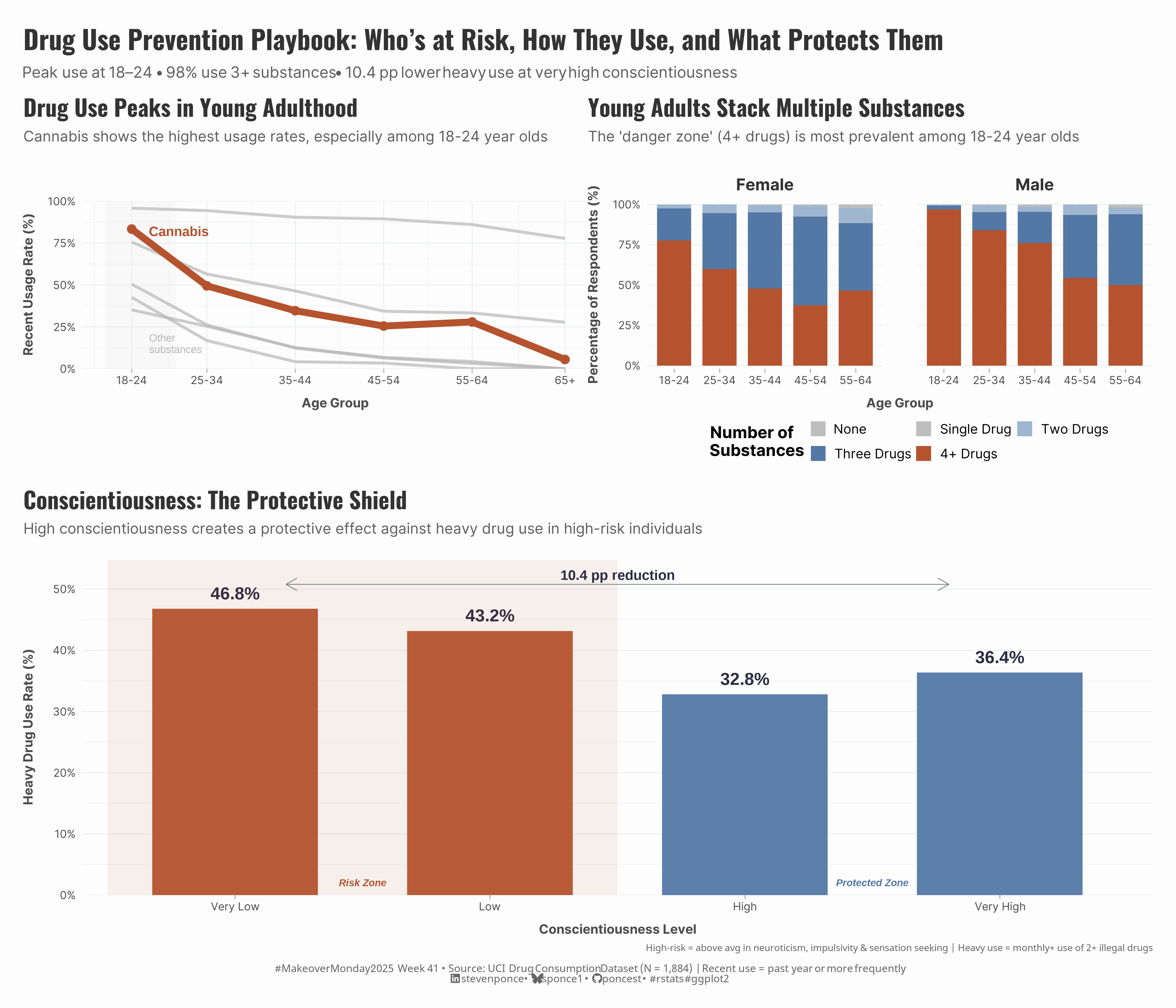
subtitle: "Peak use at 18–24 • 98% use 3+ substances • 10.4 pp lower heavy use at very high conscientiousness"
description: "Young adults (18-24) show peak polydrug use, but conscientiousness offers a protective shield—reducing heavy drug use by 22% among high-risk individuals. A data-driven exploration using the UCI Drug Consumption dataset."
date: "2025-10-21"
categories: ["MakeoverMonday", "2025"]
tags: [
"makeover-monday",
"data-visualization",
"ggplot2",
"public-health",
"substance-use",
"personality-psychology",
"risk-factors",
"polydrug-use",
"conscientiousness",
"young-adults",
"tidyverse",
"patchwork",
"uci-dataset"
]
image: "thumbnails/mm_2025_41.png"
format:
html:
toc: true
toc-depth: 5
code-link: true
code-fold: true
code-tools: true
code-summary: "Show code"
editor_options:
chunk_output_type: inline
execute:
freeze: true
cache: true
error: false
message: false
warning: false
eval: true
---
```{r}
#| label: setup-links
#| include: false
# CENTRALIZED LINK MANAGEMENT
## Project-specific info
current_year <- 2025
current_week <- 41
project_file <- "mm_2025_41.qmd"
project_image <- "mm_2025_41.png"
## Data Sources
data_main <- "https://data.world/makeovermonday/2025-week-41-drug-consumptions-uci0"
data_secondary <- "https://archive.ics.uci.edu/dataset/373/drug+consumption+quantified"
## Repository Links
repo_main <- "https://github.com/poncest/personal-website/"
repo_file <- paste0("https://github.com/poncest/personal-website/blob/master/data_visualizations/MakeoverMonday/", current_year, "/", project_file)
## External Resources/Images
chart_original <- "https://raw.githubusercontent.com/poncest/MakeoverMonday/refs/heads/master/2025/Week_41/original_chart.png"
## Organization/Platform Links
org_primary <- "https://www.kaggle.com/datasets/obeykhadija/drug-consumptions-uci?resource=download"
org_secondary <- "https://archive.ics.uci.edu/dataset/373/drug+consumption+quantified"
# Helper function to create markdown links
create_link <- function(text, url) {
paste0("[", text, "](", url, ")")
}
# Helper function for citation-style links
create_citation_link <- function(text, url, title = NULL) {
if (is.null(title)) {
paste0("[", text, "](", url, ")")
} else {
paste0("[", text, "](", url, ' "', title, '")')
}
}
```
### Original
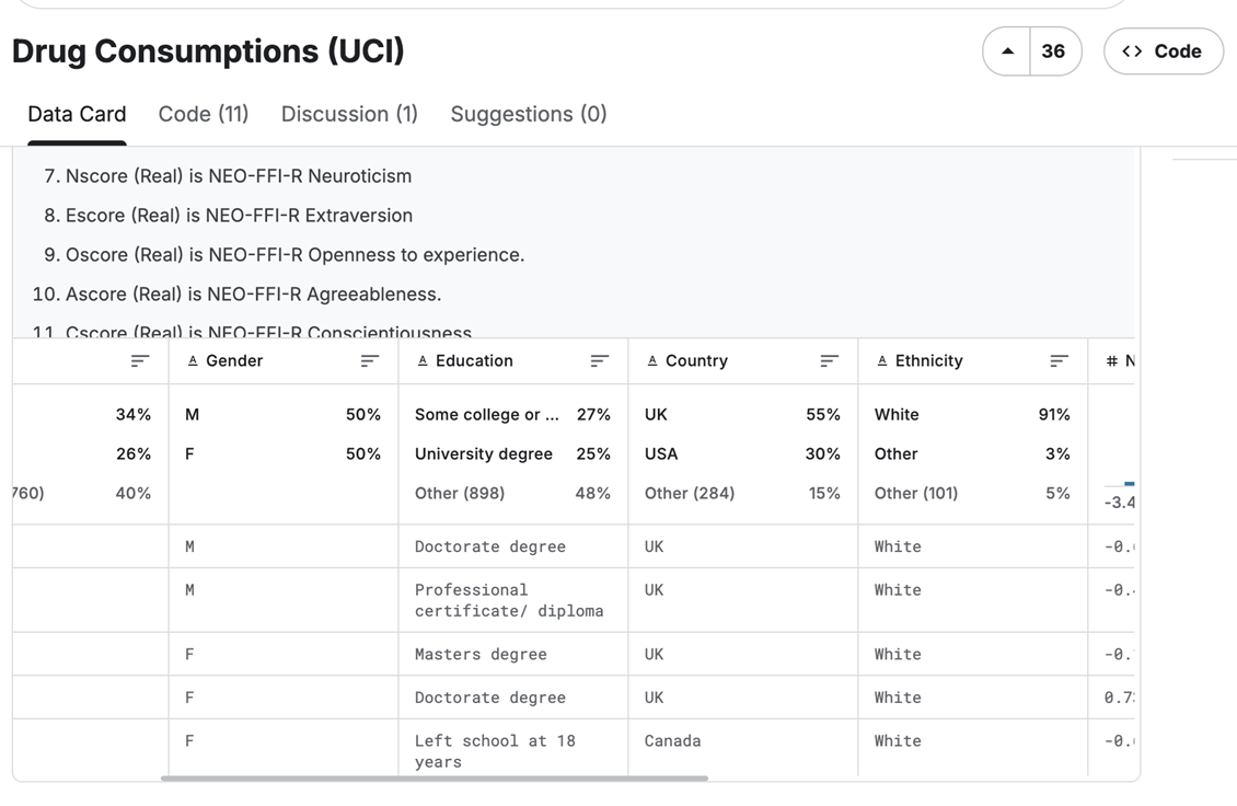
The original visualization comes from `r create_link("Drug Consumptions (UCI)", data_secondary)`
<!--  -->
### Makeover
{#fig-1}
### <mark> **Steps to Create this Graphic** </mark>
#### 1. Load Packages & Setup
```{r}
#| label: load
#| warning: false
#| message: false
#| results: "hide"

## 1. LOAD PACKAGES & SETUP ----
suppressPackageStartupMessages({
  if (!require("pacman")) install.packages("pacman")
  pacman::p_load(
    tidyverse,  # Easily Install and Load the 'Tidyverse'
    ggtext,     # Improved Text Rendering Support for 'ggplot2'
    showtext,   # Using Fonts More Easily in R Graphs
    scales,     # Scale Functions for Visualization
    glue,       # Interpreted String Literals
    patchwork   # Using Fonts More Easily in R Graphs
  )
})

### |- figure size ----
camcorder::gg_record(
    dir    = here::here("temp_plots"),
    device = "png",
    width  = 14,
    height = 12,
    units  = "in",
    dpi    = 320
)

# Source utility functions
suppressMessages(source(here::here("R/utils/fonts.R")))
source(here::here("R/utils/social_icons.R"))
source(here::here("R/utils/image_utils.R"))
source(here::here("R/themes/base_theme.R"))
```
#### 2. Read in the Data
```{r}
#| label: read
#| include: true
#| eval: true
#| warning: false
#|
drug_consumption_raw <- read_csv(
  here::here('data/MakeoverMonday/2025/Drug_Consumption.csv')) |>
  janitor::clean_names()
```
#### 3. Examine the Data
```{r}
#| label: examine
#| include: true
#| eval: true
#| results: 'hide'
#| warning: false

glimpse(drug_consumption_raw)
skimr::skim_without_charts(drug_consumption_raw)
```
#### 4. Tidy Data
```{r}
#| label: tidy
#| warning: false

drug_consumption <- drug_consumption_raw |>
  mutate(
    across(alcohol:vsa, ~ case_when(
      .x == "CL0" ~ 0, .x == "CL1" ~ 1, .x == "CL2" ~ 2,
      .x == "CL3" ~ 3, .x == "CL4" ~ 4, .x == "CL5" ~ 5,
      .x == "CL6" ~ 6, TRUE ~ NA_real_
    ))
  )

### |- P1: Age trajectory data ----
age_trajectory_data <- drug_consumption |>
  select(age, cannabis, alcohol, nicotine, coke, ecstasy, lsd) |>
  mutate(age_numeric = case_when(
    age == "18-24" ~ 21, age == "25-34" ~ 29.5, age == "35-44" ~ 39.5,
    age == "45-54" ~ 49.5, age == "55-64" ~ 59.5, age == "65+" ~ 70
  )) |>
  pivot_longer(
    cannabis:lsd,
    names_to = "substance",
    values_to = "usage"
  ) |>
  filter(!is.na(age_numeric)) |>
  group_by(age_numeric, age, substance) |>
  summarise(
    pct_recent = mean(usage >= 3, na.rm = TRUE) * 100,
    .groups = "drop"
  ) |>
  mutate(
    substance = factor(substance,
      levels = c("cannabis", "alcohol", "nicotine", "coke", "ecstasy", "lsd"),
      labels = c("Cannabis", "Alcohol", "Nicotine", "Cocaine", "Ecstasy", "LSD")
    ),
    highlight = substance == "Cannabis"
  )

### |- P2: Polydrugs patterns data ----
polydrug_data <- drug_consumption |>
  select(id, age, gender, alcohol:vsa) |>
  filter(age != "65+") |>
  pivot_longer(
    alcohol:vsa,
    names_to = "drug",
    values_to = "level"
  ) |>
  filter(drug != "semer") |>
  mutate(recent_use = if_else(level >= 3, 1, 0)) |>
  group_by(id, age, gender) |>
  summarise(
    num_drugs = sum(recent_use, na.rm = TRUE),
    .groups = "drop"
  ) |>
  mutate(
    polydrug_category = case_when(
      num_drugs == 0 ~ "None",
      num_drugs == 1 ~ "Single Drug",
      num_drugs == 2 ~ "Two Drugs",
      num_drugs == 3 ~ "Three Drugs",
      num_drugs >= 4 ~ "4+ Drugs"
    ),
    polydrug_category = factor(polydrug_category,
      levels = c(
        "None", "Single Drug", "Two Drugs",
        "Three Drugs", "4+ Drugs"
      )
    ),
    age = factor(age, levels = c("18-24", "25-34", "35-44", "45-54", "55-64"))
  )

### |- P2a: Headline metrics for polydrug use (3+ substances) ----
polydrug_summary <- polydrug_data |>
  count(age, gender, polydrug_category, name = "n") |>
  group_by(age, gender) |>
  mutate(p = n / sum(n)) |>
  summarise(
    share_3plus = sum(p[polydrug_category %in% c("Three Drugs", "4+ Drugs")]),
    .groups = "drop"
  )

# Overall headline for the youngest group (used in the global subtitle)
share_3plus_18_24_overall <- polydrug_summary |>
  filter(age == "18-24") |>
  summarise(value = mean(share_3plus, na.rm = TRUE)) |>
  pull(value)

# Calculate 3+ drug percentages for annotation
p2_labels <- polydrug_data |>
  count(age, gender, polydrug_category) |>
  group_by(age, gender) |>
  mutate(pct = n / sum(n) * 100) |>
  filter(polydrug_category %in% c("Three Drugs", "4+ Drugs")) |>
  group_by(age, gender) |>
  summarise(
    pct_3plus = sum(pct),
    .groups = "drop"
  )

### |- P3: Conscientiousness data ----
conscientiousness_data <- drug_consumption |>
  mutate(
    high_risk = (nscore > 0) & (impulsive > 0) & (ss > 0),
    cscore_category = case_when(
      cscore < quantile(cscore, 0.25, na.rm = TRUE) ~ "Very Low",
      cscore < quantile(cscore, 0.5, na.rm = TRUE) ~ "Low",
      cscore < quantile(cscore, 0.75, na.rm = TRUE) ~ "High",
      TRUE ~ "Very High"
    ),
    cscore_category = factor(cscore_category,
      levels = c("Very Low", "Low", "High", "Very High")
    )
  ) |>
  rowwise() |>
  mutate(
    heavy_illegal = sum(c(
      cannabis, coke, ecstasy, lsd, mushrooms,
      ketamine, amphet
    ) >= 4, na.rm = TRUE) >= 2
  ) |>
  ungroup() |>
  filter(high_risk) |>
  group_by(cscore_category) |>
  summarise(
    pct_heavy_use = mean(heavy_illegal, na.rm = TRUE) * 100,
    n = n(),
    .groups = "drop"
  )

# Calculate reduction
reduction_pp <- conscientiousness_data$pct_heavy_use[1] -
  conscientiousness_data$pct_heavy_use[4]
```
#### 5. Visualization Parameters
```{r}
#| label: params
#| include: true
#| warning: false

### |-  plot aesthetics ----
# Get base colors with custom palette
colors <- get_theme_colors(
  palette = list(
    danger        = "#B5532F",
    primary       = "#1E3A5F",
    neutral_dark  = "#5378A6",
    neutral_mid   = "#9FB6D0",
    neutral_light = "#E8E8E8",
    other_lines   = "#B8B8B8",
    text_primary  = "#2B2D42",
    text_secondary= "#6C757D"
    )
  )

### |-  titles and caption ----
title_text <- str_glue("Drug Use Prevention Playbook: Who’s at Risk, How They Use, and What Protects Them")

subtitle_text <- str_glue(
    "Peak use at 18–24 • {scales::percent(share_3plus_18_24_overall, accuracy = 1)} use 3+ substances • ",
    "{sprintf('%.1f', reduction_pp)} pp lower heavy use at very high conscientiousness"
  )

# Create caption
caption_text <- create_mm_caption(
  mm_year = current_year,
  mm_week = current_week,
  source_text = "UCI Drug Consumption Dataset (N = 1,884) | Recent use = past year or more frequently"
)

### |-  fonts ----
setup_fonts()
fonts <- get_font_families()

### |-  plot theme ----

# Start with base theme
base_theme <- create_base_theme(colors)

# Add weekly-specific theme elements
weekly_theme <- extend_weekly_theme(
  base_theme,
  theme(
    # # Text styling
    plot.title = element_text(
      size = rel(1.4), family = fonts$title, face = "bold",
      color = colors$title, lineheight = 1.1, hjust = 0,
      margin = margin(t = 5, b = 10)
    ),
    plot.subtitle = element_text(
      size = rel(0.9), family = fonts$subtitle, face = "italic",
      color = alpha(colors$subtitle, 0.9), lineheight = 1.1,
      margin = margin(t = 0, b = 20)
    ),

    # Legend formatting
    legend.position = "plot",
    legend.justification = "top",
    legend.margin = margin(l = 12, b = 5),
    legend.key.size = unit(0.8, "cm"),
    legend.box.margin = margin(b = 10),
    legend.title = element_text(face = "bold"),

    # Axis formatting
    axis.ticks.y = element_blank(),
    axis.ticks.x = element_line(color = "gray", linewidth = 0.5),
    axis.title.x = element_text(
      face = "bold", size = rel(0.85),
      margin = margin(t = 10)
    ),
    axis.title.y = element_text(
      face = "bold", size = rel(0.85),
      margin = margin(r = 10)
    ),
    axis.text.x = element_text(
      size = rel(0.85), family = fonts$subtitle,
      color = colors$text
    ),
    axis.text.y = element_text(
      size = rel(0.85), family = fonts$subtitle,
      color = colors$text
    ),

    # Grid lines
    panel.grid.minor = element_line(color = "#ecf0f1", linewidth = 0.2),
    panel.grid.major = element_line(color = "#ecf0f1", linewidth = 0.4),

    # Margin
    plot.margin = margin(20, 20, 20, 20)
  )
)

# Set theme
theme_set(weekly_theme)
```
#### 6. Plot
```{r}
#| label: plot
#| warning: false

### |- P1: Age trajectory chart ----
p1 <-
ggplot() +
  # Annotate
  annotate("rect", xmin=18, xmax=26, ymin=0, ymax=100,
           fill="#EDEDED", color=NA, alpha=0.35) +
  annotate("text",
    x = 22, y = 95, label = "Peak Risk\nAge Group",
    color = colors$text_secondary, size = 3, fontface = "italic", lineheight = 0.9
  ) +
  annotate("text",
           x = 23, y = 82, label = "Cannabis",
           color = colors$palette$danger, fontface = "bold", size = 4, hjust = 0
  ) +
  annotate("text",
           x = 23, y = 15, label = "Other\nsubstances",
           color = colors$palette$other_lines, size = 3.2, hjust = 0, lineheight = 0.9
  ) +
  # Geoms
  geom_line(
    data = filter(age_trajectory_data, !highlight),
    aes(age_numeric, pct_recent, group = substance),
    color = colors$palette$other_lines, linewidth = 1.2, alpha = 0.7
  ) +
  geom_line(
    data = filter(age_trajectory_data, highlight),
    aes(age_numeric, pct_recent, group = substance),
    color = colors$palette$danger, linewidth = 2.8
  ) +
  geom_point(
    data = filter(age_trajectory_data, highlight),
    aes(age_numeric, pct_recent),
    size = 3.2, color = colors$palette$danger
  ) +
  # Scales
  scale_x_continuous(
    breaks = c(21, 29.5, 39.5, 49.5, 59.5, 70),
    labels = c("18-24", "25-34", "35-44", "45-54", "55-64", "65+")
  ) +
  scale_y_continuous(
    labels = function(x) paste0(x, "%"),
    limits = c(0, 100), expand = c(0, 0)
  ) +
  # Labs
  labs(
    title = "Drug Use Peaks in Young Adulthood",
    subtitle = "Cannabis shows the highest usage rates, especially among 18-24 year olds",
    x = "Age Group",
    y = "Recent Usage Rate (%)"
  ) +
  # Theme
  theme(
    plot.margin = margin(0, 0, 0, 0)
  )

### |- P2: Polydrugs patterns chart ----
p2 <-
ggplot(polydrug_data, aes(age, fill = polydrug_category)) +
  # Geoms
  geom_bar(position = "fill", width = 0.75) +
  # Scales
  scale_y_continuous(labels = percent_format(), expand = c(0, 0.02)) +
  scale_fill_manual(values = c(
    "None"        = "gray",
    "Single Drug" = "gray",
    "Two Drugs"   = colors$palette$neutral_mid,
    "Three Drugs" = colors$palette$neutral_dark,
    "4+ Drugs"    = colors$palette$danger
  )) +
  coord_cartesian(clip = "off", ylim = c(0, 1)) +
  # labs
  labs(
    title = "Young Adults Stack Multiple Substances",
    subtitle = "The 'danger zone' (4+ drugs) is most prevalent among 18-24 year olds",
    x = "Age Group",
    y = "Percentage of Respondents (%)",
    fill = "Number of\nSubstances"
  ) +
  # Facets
  facet_wrap(~gender, labeller = labeller(gender = c(F = "Female", M = "Male"))) +
  # Theme
  theme(
    legend.position = "bottom",
    legend.justification = "top",
    legend.key.size = unit(0.5, "cm"),
    strip.text = element_text(
      face = "bold",
      color = "gray20",
      size = rel(1),
      margin = margin(t = 8, b = 8)
    ),
    panel.spacing = unit(2, "lines"),
    plot.margin = margin(0, 0, 0, 0)
  ) +
  guides(fill = guide_legend(nrow = 2, byrow = TRUE))

### |- P3: Conscientiousness chart ----
p3 <-
ggplot(
  conscientiousness_data,
  aes(cscore_category, pct_heavy_use)
) +
  # Geoms
  geom_col(aes(fill = cscore_category), width = 0.65, alpha = 0.95) +
  geom_text(aes(label = sprintf("%.1f%%", pct_heavy_use)),
    vjust = -0.8, fontface = "bold", size = 5.2,
    color = colors$palette$text_primary
  ) +
  # Annotate
  annotate("rect",
    xmin = 0.5, xmax = 2.5, ymin = 0, ymax = Inf,
    fill = alpha(colors$palette$danger, 0.08), color = NA
  ) +
  annotate("segment",
    x = 1.2, xend = 3.8,
    y = max(conscientiousness_data$pct_heavy_use) + 4,
    yend = max(conscientiousness_data$pct_heavy_use) + 4,
    arrow = arrow(ends = "both", length = unit(0.15, "inches")),
    color = colors$palette$text_secondary, linewidth = 0.3
  ) +
  annotate("text",
    x = 2.5,
    y = max(conscientiousness_data$pct_heavy_use) + 5.5,
    label = sprintf("%.1f pp reduction", reduction_pp),
    fontface = "bold", size = 4.2, color = colors$palette$text_primary
  ) +
  annotate("text",
    x = 1.5, y = 2, label = "Risk Zone",
    color = colors$palette$danger, fontface = "bold.italic", size = 3
  ) +
  annotate("text",
    x = 3.5, y = 2, label = "Protected Zone",
    color = colors$palette$neutral_dark, fontface = "bold.italic", size = 3
  ) +
  # Scales
  scale_fill_manual(values = c(
    "Very Low" = colors$palette$danger,
    "Low" = colors$palette$danger,
    "High" = colors$palette$neutral_dark,
    "Very High" = colors$palette$neutral_dark
  )) +
  scale_y_continuous(
    labels = function(x) paste0(x, "%"),
    limits = c(0, max(conscientiousness_data$pct_heavy_use) + 8),
    expand = c(0, 0)
  ) +
  # Labs
  labs(
    title = "Conscientiousness: The Protective Shield",
    subtitle = "High conscientiousness creates a protective effect against heavy drug use in high-risk individuals",
    x = "Conscientiousness Level",
    y = "Heavy Drug Use Rate (%)",
    caption = "High-risk = above avg in neuroticism, impulsivity & sensation seeking | Heavy use = monthly+ use of 2+ illegal drugs"
  ) +
  # Theme
  theme(
    panel.grid.major.x = element_blank(),
    plot.caption = element_text(lineheight = 1.3, size = 8, family = fonts$caption, color = colors$caption),
    plot.margin = margin(0, 0, 0, 0)
  )

### |- Combined Plots ----
combined_plots <- (p1 | p2) / p3 +
  plot_layout(heights = c(1, 2))

combined_plots <- combined_plots +
  plot_annotation(
    title = title_text,
    subtitle = subtitle_text,
    caption = caption_text,
    theme = theme(
      plot.title = element_text(
        size = rel(1.6),
        family = fonts$title,
        face = "bold",
        color = colors$title,
        lineheight = 1.1,
        margin = margin(t = 5, b = 5)
      ),
      plot.subtitle = element_markdown(
        size = rel(0.95),
        family = fonts$subtitle,
        color = alpha(colors$subtitle, 0.9),
        lineheight = 1.2,
        margin = margin(t = 5, b = 10)
      ),
      plot.caption = element_markdown(
        size = rel(0.65),
        family = fonts$caption,
        color = colors$caption,
        hjust = 0.5,
        margin = margin(t = 10)
      )
    )
  )
```
#### 7. Save
```{r}
#| label: save
#| warning: false

### |-  plot image ----
save_plot_patchwork(
  plot = combined_plots,
  type = "makeovermonday",
  year = current_year,
  week = current_week,
  width = 14,
  height = 12
  )
```
#### 8. Session Info
::: {.callout-tip collapse="true"}
##### Expand for Session Info
```{r, echo = FALSE}
#| eval: true
#| warning: false
sessionInfo()
```
:::
#### 9. GitHub Repository
::: {.callout-tip collapse="true"}
##### Expand for GitHub Repo
The complete code for this analysis is available in `r create_link(project_file, repo_file)`.
For the full repository, `r create_link("click here", repo_main)`.
:::
#### 10. References
::: {.callout-tip collapse="true"}
##### Expand for References
1. Data:
- Makeover Monday `r current_year` Week `r current_week`: `r create_link("Drug Consumptions (UCI)", data_main)`
2. Article
- `r create_link("Drug Consumptions (UCI)", data_secondary)`
3. Research Paper:
- Fehrman, E., Muhammad, A. K., Mirkes, E. M., Egan, V., & Gorban, A. N. (2015). The Five Factor Model of personality and evaluation of drug consumption risk. arXiv preprint. `r create_link("arXiv:1506.06297", "https://arxiv.org/abs/1506.06297")`
:::
#### 11. Custom Functions Documentation
::: {.callout-note collapse="true"}
##### 📦 Custom Helper Functions
This analysis uses custom functions from my personal module library for efficiency and consistency across projects.
**Functions Used:**
- **`fonts.R`**: `setup_fonts()`, `get_font_families()` - Font management with showtext
- **`social_icons.R`**: `create_social_caption()` - Generates formatted social media captions
- **`image_utils.R`**: `save_plot()` - Consistent plot saving with naming conventions
- **`base_theme.R`**: `create_base_theme()`, `extend_weekly_theme()`, `get_theme_colors()` - Custom ggplot2 themes
**Why custom functions?**\
These utilities standardize theming, fonts, and output across all my data visualizations. The core analysis (data tidying and visualization logic) uses only standard tidyverse packages.
**Source Code:**\
View all custom functions → [GitHub: R/utils](https://github.com/poncest/personal-website/tree/master/R)
:::

