---
title: "Youth Vaping Crisis: Policy Intervention Failure"
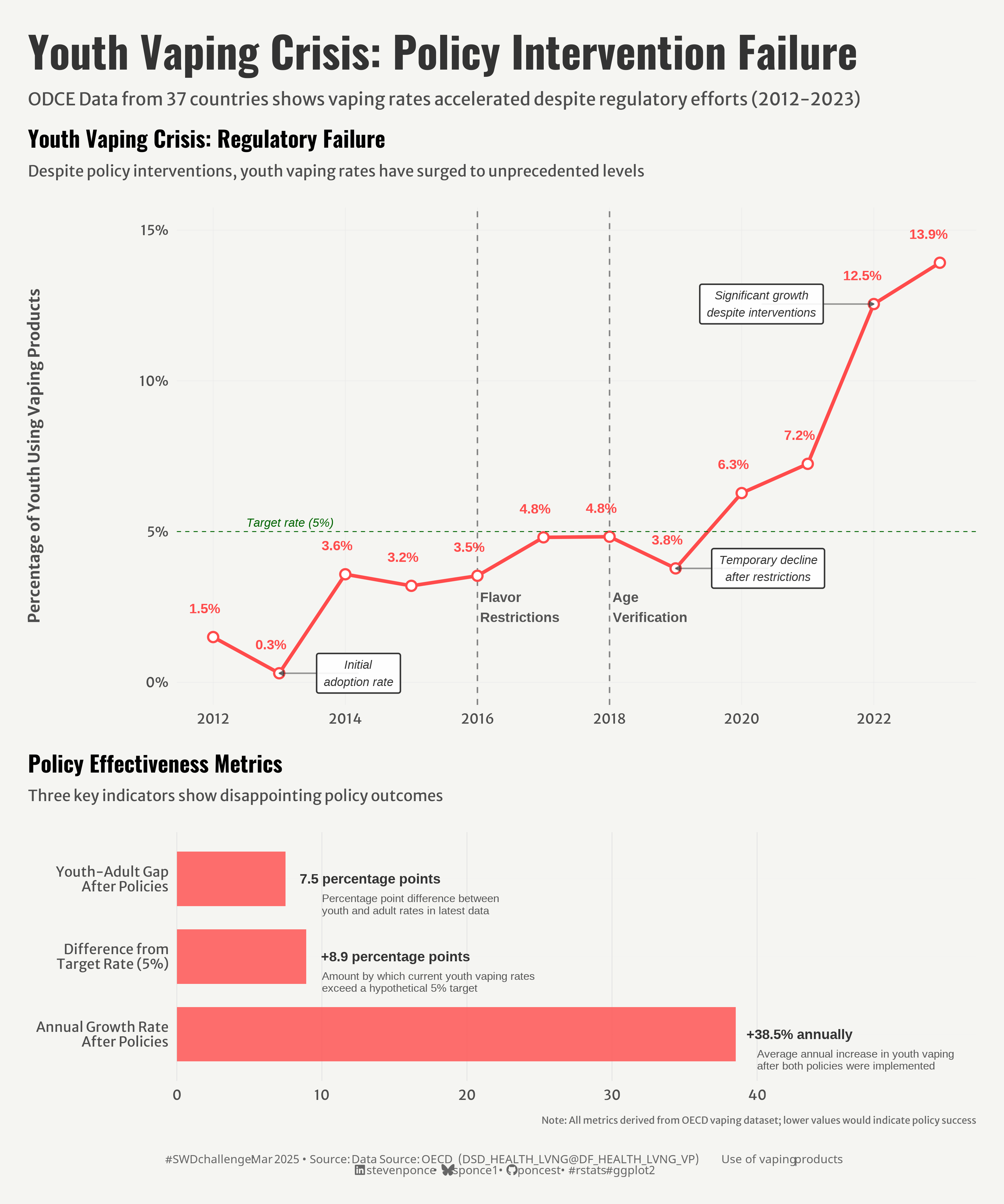
subtitle: "ODCE Data from 37 countries shows vaping rates accelerated despite regulatory efforts (2012-2023)"
description: "This visualization examines the failure of vaping regulations to curb youth adoption rates. Using OECD data from 37 countries, the analysis reveals how policy interventions implemented in 2016 and 2018 failed to prevent the alarming rise in youth vaping, with rates surging from 0.3% to 13.9% over a decade despite regulatory efforts."
author: "Steven Ponce"
date: "2025-03-02"
categories: ["SWDchallenge", "2025"]
tags: [
"vaping", "public health", "policy analysis", "youth health", "regulatory failure", "data storytelling", "ggplot2", "disappointing results", "trend analysis", "health policy"
]
image: "thumbnails/swd_2025_03.png"
format:
html:
toc: true
toc-depth: 5
code-link: true
code-fold: true
code-tools: true
code-summary: "Show code"
editor_options:
chunk_output_type: inline
execute:
freeze: true
cache: true
error: false
message: false
warning: false
eval: true
# share:
# permalink: "https://stevenponce.netlify.app/data_visualizations/SWD Challenge/2025/swd_2025_03.html"
# description: "Analysis of OECD data reveals how youth vaping rates surged despite regulatory interventions, highlighting a critical public health policy failure"
# linkedin: true
# twitter: true
# email: true
---
{#fig-1}
### <mark> __Steps to Create this Graphic__ </mark>
#### 1. Load Packages & Setup
```{r}
#| label: load
if (!require("pacman")) install.packages("pacman")
pacman::p_load(
  tidyverse,         # Easily Install and Load the 'Tidyverse'
  ggtext,            # Improved Text Rendering Support for 'ggplot2'
  showtext,          # Using Fonts More Easily in R Graphs
  scales,            # Scale Functions for Visualization
  glue,              # Interpreted String Literals
  here,              # A Simpler Way to Find Your Files
  janitor,           # Simple Tools for Examining and Cleaning Dirty Data
  skimr,             # Compact and Flexible Summaries of Data
  patchwork,         # The Composer of Plots
  camcorder          # Record Your Plot History
)

### |- figure size ----
gg_record(
  dir    = here::here("temp_plots"),
  device = "png",
  width  = 10,
  height = 12,
  units  = "in",
  dpi    = 320)

# Source utility functions
suppressMessages(source(here::here("R/utils/fonts.R")))
source(here::here("R/utils/social_icons.R"))
source(here::here("R/utils/image_utils.R"))
source(here::here("R/themes/base_theme.R"))
```
#### 2. Read in the Data
```{r}
#| label: read
vaping_raw <- read_csv(
  here::here("data/OECD_use_of_vaping_products.csv")
  ) |>
  clean_names()
```
#### 3. Examine the Data
```{r}
#| label: examine
#| include: true
#| eval: true
#| results: 'hide'
#| warning: false
glimpse(vaping_raw)
skim(vaping_raw)
```
#### 4. Tidy Data
```{r}
#| label: tidy
vaping_clean <- vaping_raw |>
  # Select only the relevant columns
  select(
    country = reference_area,
    year = time_period,
    age_group = age_2,
    sex = sex_2,
    vaping_percentage = obs_value,
    data_status = observation_status
  ) |>
  # Filter for valid data
  filter(!is.na(vaping_percentage)) |>
  mutate(
    year = as.numeric(year),
    # Clean up the age group labels for better visualization
    age_group = case_when(
      age_group == "15 years or over" ~ "Adults (15+)",
      age_group == "15-24 years" ~ "From 15 to 24 years",
      TRUE ~ age_group
    ),
    # Clean up sex labels
    sex = case_when(
      sex == "_T" ~ "Total",
      sex == "M" ~ "Male",
      sex == "F" ~ "Female",
      TRUE ~ sex
    )
  )

# Get main trend data for youth vaping
youth_trend <- vaping_clean |>
  filter(
    age_group == "From 15 to 24 years",
    sex == "Total"
  ) |>
  group_by(year) |>
  summarize(
    avg_vaping = mean(vaping_percentage, na.rm = TRUE),
    .groups = "drop")

# Define policies and their implementation dates
policy_years <- c(2016, 2018)
policy_labels <- c("Flavor\nRestrictions", "Age\nVerification")

policy_data <- tibble(
  year = policy_years,
  policy = policy_labels,
  y_pos = c(2, 2)
)

# Calculate key metrics from the data for annotations
annotations <- youth_trend |>
  # Calculate year-over-year change
  arrange(year) |>
  mutate(
    prev_value = lag(avg_vaping),
    pct_change = (avg_vaping - prev_value) / prev_value * 100
  ) |>
  # Select key years for annotations
  filter(year %in% c(2013, 2016, 2019, 2022)) |>
  mutate(
    # Create annotation text with proper placement coordinates
    label = case_when(
      year == 2013 ~ "Initial\nadoption rate",
      year == 2016 ~ "",
      year == 2019 ~ "Temporary decline\nafter restrictions",
      year == 2022 ~ "Significant growth\ndespite interventions",
      TRUE ~ ""
    ),
    # Adjust label positions
    x_pos = case_when(
      year == 2013 ~ year + 1.2,
      year == 2019 ~ year + 1.4,
      year == 2022 ~ year - 1.7,
      TRUE ~ year
    ),
    y_pos = case_when(
      year == 2013 ~ avg_vaping,
      year == 2019 ~ avg_vaping,
      year == 2022 ~ avg_vaping,
      TRUE ~ avg_vaping
    ),
    # Calculate growth since policy implementation
    growth_since_policy = if_else(
      year == 2022,
      (avg_vaping / youth_trend$avg_vaping[youth_trend$year == 2016] - 1) * 100,
      NA_real_
    )
  )

# Calculate the growth percentage for 2022 annotation
growth_pct <- round(annotations$growth_since_policy[annotations$year == 2022], 0)

# Calculate growth rates by period
period_growth <- youth_trend |>
  mutate(
    period = case_when(
      year <= 2016 ~ "Pre-Policy (2012-2016)",
      year > 2016 & year <= 2018 ~ "Initial Response (2016-2018)",
      year > 2018 ~ "Post-Implementation (2018-2022)",
      TRUE ~ "Other"
    )
  ) |>
  group_by(period) |>
  summarize(
    start_year = min(year),
    end_year = max(year),
    start_value = first(avg_vaping),
    end_value = last(avg_vaping),
    # Calculate annualized growth rate for fair comparison
    years_elapsed = end_year - start_year,
    total_growth = (end_value / start_value - 1) * 100,
    annual_growth = (((end_value / start_value)^(1/years_elapsed)) - 1) * 100,
    .groups = "drop"
  ) |>
  # Filter out any incomplete periods
  filter(years_elapsed > 0) |>
  # Add a period order for plotting
  mutate(period_order = case_when(
    period == "Pre-Policy (2012-2016)" ~ 1,
    period == "Initial Response (2016-2018)" ~ 2,
    period == "Post-Implementation (2018-2022)" ~ 3,
    TRUE ~ 4
  )) |>
  arrange(period_order)

# Calculate age group gap over time
age_gap_data <- vaping_clean |>
  filter(sex == "Total") |>
  group_by(year, age_group) |>
  summarize(avg_vaping = mean(vaping_percentage, na.rm = TRUE), .groups = "drop") |>
  pivot_wider(names_from = age_group, values_from = avg_vaping) |>
  rename(
    youth = `From 15 to 24 years`,
    adults = `Adults (15+)`
  ) |>
  mutate(
    gap = youth - adults,
    gap_pct = (youth / adults - 1) * 100
  ) |>
  # Calculate the change in gap size over time
  arrange(year) |>
  mutate(
    period = case_when(
      year <= 2016 ~ "Pre-Policy",
      year > 2016 & year <= 2018 ~ "Initial Response",
      year > 2018 ~ "Post-Implementation",
      TRUE ~ "Other"
    )
  )

# Calculate policy effectiveness metrics
policy_effectiveness <- tibble(
  metric = c(
    "Annual Growth Rate After Policies",
    "Youth-Adult Gap After Policies",
    "Difference from Target Rate (5%)"
  ),
  value = c(
    # Annual growth rate after policy implementation (2018-2022)
    period_growth$annual_growth[period_growth$period == "Post-Implementation (2018-2022)"],

    # Current youth-adult gap (latest year)
    age_gap_data$gap[age_gap_data$year == max(age_gap_data$year)],

    # Difference from a hypothetical target rate of 5% (latest year data)
    youth_trend$avg_vaping[youth_trend$year == max(youth_trend$year)] - 5
  ),
  description = c(
    "Average annual increase in youth vaping\nafter both policies were implemented",
    "Percentage point difference between\nyouth and adult rates in latest data",
    "Amount by which current youth vaping rates\nexceed a hypothetical 5% target"
  )
)

policy_effectiveness <- policy_effectiveness |>
  mutate(
    # Reorder factors for display
    metric = factor(metric, levels = rev(metric)),
    # Category labels
    metric_label = case_when(
      metric == "Annual Growth Rate After Policies" ~ "Annual Growth Rate\nAfter Policies",
      metric == "Youth-Adult Gap After Policies" ~ "Youth-Adult Gap\nAfter Policies",
      metric == "Difference from Target Rate (5%)" ~ "Difference from\nTarget Rate (5%)",
      TRUE ~ as.character(metric)
    ),
    # Format value labels
    value_label = case_when(
      metric == "Annual Growth Rate After Policies" ~ paste0("+", round(value, 1), "% annually"),
      metric == "Youth-Adult Gap After Policies" ~ paste0(round(value, 1), " percentage points"),
      metric == "Difference from Target Rate (5%)" ~ paste0("+", round(value, 1), " percentage points"),
      TRUE ~ as.character(round(value, 1))
    )
  )

# Create separate data frames for the description texts
desc_data1 <- policy_effectiveness |>
  filter(metric != "Annual Growth Rate After Policies")

desc_data2 <- policy_effectiveness |>
  filter(metric == "Annual Growth Rate After Policies")
```
#### 5. Visualization Parameters
```{r}
#| label: params
### |-  plot aesthetics ----
# Get base colors with custom palette
colors <- get_theme_colors(palette = c(
  "#FF4B4B", "#555555", "#333333"
  ))

### |-  titles and caption ----
title_text   <- str_glue("Youth Vaping Crisis: Policy Intervention Failure")
subtitle_text <- str_glue("ODCE Data from 37 countries shows vaping rates accelerated despite regulatory efforts (2012-2023)")

# Create caption
caption_text <- create_swd_caption(
    year = 2025,
    month = "Mar",
    source_text = "Data Source: OECD (DSD_HEALTH_LVNG@DF_HEALTH_LVNG_VP) Use of vaping products"
  )


# |- fonts ----
setup_fonts()
fonts <- get_font_families()

### |-  plot theme ----
# Start with base theme
base_theme <- create_base_theme(colors)

# Add weekly-specific theme elements
weekly_theme <- extend_weekly_theme(
  base_theme,
  theme(
    # Text styling
    plot.title = element_text(face = "bold", family = fonts$title, size = rel(1.14), margin = margin(b = 10)),
    plot.subtitle = element_text(family = fonts$subtitle, color = colors$text, size = rel(0.78), margin = margin(b = 20)),

    # Axis elements
    axis.title = element_text(color = colors$text, size = rel(0.8)),
    axis.text = element_text(color = colors$text, size = rel(0.7)),

    # Grid elements
    panel.grid.minor = element_blank(),
    panel.grid.major = element_line(color = "grey95", linewidth = 0.1),

    # Legend elements
    legend.position = "plot",
    legend.title = element_text(family = fonts$text, size = rel(0.8)),
    legend.text = element_text(family = fonts$text, size = rel(0.7)),

    # Plot margins
    plot.margin = margin(t = 10, r = 10, b = 10, l = 10),
  )
)

# Set theme
theme_set(weekly_theme)
```
#### 6. Plot
```{r}
#| label: plot
### |-  P1. Vaping Trend Plot  ----
vaping_tred <- youth_trend |>
  ggplot(aes(x = year, y = avg_vaping)) +
  # Geoms
  geom_hline(yintercept = seq(0, 15, by = 5), color = 'gray90', linewidth = 0.1) +
  geom_vline(xintercept = seq(2012, 2022, by = 2), color = 'gray90', linewidth = 0.1) +

  geom_vline(xintercept = policy_years,                                         # Policy intervention lines
             linetype = "dashed", color = colors$palette[2], alpha = 0.7, size = 0.5) +

  geom_line(size = 1.2, color = colors$palette[1]) +
  geom_point(size = 3.5, color = colors$palette[1]) +
  geom_point(size = 2, color = "white") +

  geom_text(data = policy_data,                                                 # Policy labels
            aes(x = year, y = y_pos, label = policy),
            color = colors$palette[2], fontface = "bold", size = 3.5,
            hjust = 0, vjust = 0, nudge_x = 0.05) +

  geom_text(aes(label = paste0(format(avg_vaping, digits = 1), "%")),
            vjust = -2.5, hjust = 0.8, color = colors$palette[1], fontface = "bold", size = 3.5) +

  # Key trend annotations
  geom_segment(data = annotations |> filter(label != ""),
               aes(x = year, xend = x_pos, y = avg_vaping, yend = y_pos),
               color = alpha(colors$palette[3], 0.5), size = 0.5,
               arrow = arrow(length = unit(0.01, "npc"), type = "closed", ends = "first")) +

  geom_label(data = annotations |> filter(label != ""),
             aes(x = x_pos, y = y_pos, label = label),
             color = colors$palette[3], size = 3, fontface = "italic",
             fill = alpha("white", 0.9), label.size = 0.5,
             label.padding = unit(0.5, "lines")) +

  geom_hline(yintercept = 5, linetype = "dashed", color = "darkgreen", size = 0.3) +
  annotate("text", x = 2012.5, y = 5.3, label = "Target rate (5%)",             # Target reference line
           color = "darkgreen", hjust = 0, size = 3, fontface = "italic") +

  # Scales
  scale_x_continuous(
    breaks = seq(2012, 2022, by = 2),
    limits = c(2012, 2023),
    ) +
  scale_y_continuous(
    labels = function(x) paste0(x, "%"),
    breaks = seq(0, 15, by = 5),
    limits = c(0, 15)
  ) +
  coord_cartesian(clip = 'off') +

  # Labs
  labs(
    title = "Youth Vaping Crisis: Regulatory Failure",
    subtitle = "Despite policy interventions, youth vaping rates have surged to unprecedented levels",
    x = NULL,
    y = "Percentage of Youth Using Vaping Products"
  )


# P2. Policy Effectiveness Plot ----
effectiveness_plot <- ggplot(policy_effectiveness, aes(x = value, y = metric_label)) +
  # Geoms
  geom_vline(xintercept = seq(0, 40, by = 10), color = "gray90", linewidth = 0.3) +
  geom_col(fill = colors$palette[1], width = 0.7, alpha = 0.8) +
  geom_text(aes(label = value_label),
            hjust = -0.1,
            color = colors$palette[3],
            size = 3.5,
            fontface = "bold") +
  # Explanatory text
  geom_text(data = desc_data1,
            aes(x = 10, label = description),
            hjust = 0,
            vjust = 1.8,
            color = colors$palette[2],
            size = 2.8,
            lineheight = 0.9) +
  geom_text(data = desc_data2,
            aes(x = 40, label = description),
            hjust = 0,
            vjust = 1.8,
            color = colors$palette[2],
            size = 2.8,
            lineheight = 0.9) +

  # Scales
  scale_x_continuous(
    limits = c(0, max(policy_effectiveness$value) * 1.3),
    breaks = seq(0, 40, by = 10),
    expand = expansion(mult = c(0, 0.1))
  ) +
  coord_cartesian(clip = 'off') +

  # Labs
  labs(
    x = NULL,
    y = NULL,
    title = "Policy Effectiveness Metrics",
    subtitle = "Three key indicators show disappointing policy outcomes",
    caption = "Note: All metrics derived from OECD vaping dataset; lower values would indicate policy success"
  ) +

  # Theme
  theme(
    plot.caption = element_text(size = rel(0.5), color = colors$caption, margin = margin(t = 10))
  )

# Combined Plots ----
combined_plot <-vaping_tred / effectiveness_plot +
  plot_layout(heights = c(2, 1)) +
  plot_annotation(
    title = title_text,
    subtitle = subtitle_text,
    caption = caption_text,
    theme = theme(
      plot.title = element_text(
        size   = rel(2.2),
        family = fonts$title,
        face   = "bold",
        color  = colors$title,
        lineheight = 1.1,
        margin = margin(t = 5, b = 5)
      ),
      plot.subtitle = element_text(
        size   = rel(0.9),
        family = fonts$subtitle,
        color  = colors$subtitle,
        lineheight = 1.2,
        margin = margin(t = 5, b = 5)
      ),
      plot.caption = element_markdown(
        size   = rel(0.6),
        family = fonts$caption,
        color  = colors$caption,
        hjust  = 0.5,
        margin = margin(t = 10)
      ),
      plot.margin = margin(t = 20, r = 10, b = 20, l = 10),
    )
  )
```
#### 7. Save
```{r}
#| label: save
### |-  plot image ----

source(here::here("R/image_utils.R"))
save_plot_patchwork(
  combined_plot, type = 'swd', year = 2025, month = 03,
  width = 10, height = 12
  )
```
#### 8. Session Info
::: {.callout-tip collapse="true"}
##### Expand for Session Info
```{r, echo = FALSE}
#| eval: true
#| warning: false
sessionInfo()
```
:::
#### 9. GitHub Repository
::: {.callout-tip collapse="true"}
##### Expand for GitHub Repo
The complete code for this analysis is available in [`swd_2025_03.qmd`](https://github.com/poncest/personal-website/tree/master/data_visualizations/SWD%20Challenge/2025/swd_2025_03.qmd).
For the full repository, [click here](https://github.com/poncest/personal-website/).
:::
#### 10. References
::: {.callout-tip collapse="true"}
##### Expand for References
Data Sources:
- OECD Use of vaping products: [`DSD_HEALTH_LVNG@DF_HEALTH_LVNG_VP`](https://data-explorer.oecd.org/vis?lc=en&df[ds]=dsDisseminateFinalDMZ&df[id]=DSD_HEALTH_LVNG%40DF_HEALTH_LVNG_VP&df[ag]=OECD.ELS.HD&dq=.A.....&pd=2012%2C&to[TIME_PERIOD]=false)
:::
