---
title: "Maternity Care Deserts Span Large Regions of the United States"
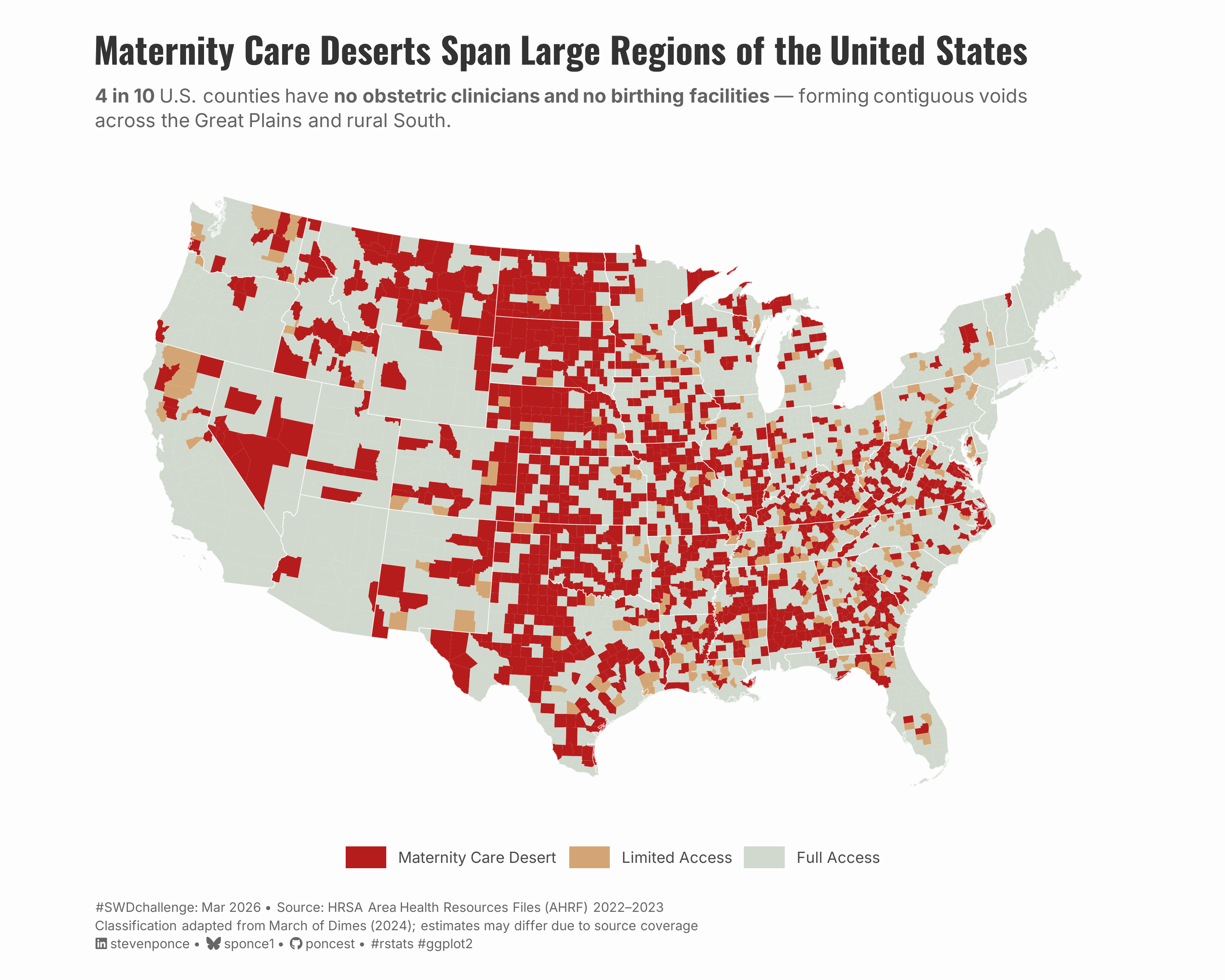
subtitle: "4 in 10 U.S. counties have no obstetric clinicians and no birthing facilities — forming contiguous voids across the Great Plains and rural South."
description: "A county-level choropleth map revealing that 4 in 10 U.S. counties have zero maternity care — no obstetric clinicians and no birthing facilities. Using HRSA Area Health Resources Files (AHRF) 2022–2023 and classification logic adapted from the March of Dimes (2024), the map demonstrates how maternity care deserts form contiguous regional voids across the Great Plains and rural South, not isolated gaps — an insight only geography can reveal."
author: "Steven Ponce"
date: "2026-03-01"
categories: ["SWDchallenge", "2026"]
tags: [
"choropleth-map",
"maternity-care",
"health-equity",
"mapping-with-purpose",
"figure-ground",
"county-level",
"public-health",
"ggplot2",
"sf",
"tigris",
"AHRF",
"March-of-Dimes"
]
image: "thumbnails/swd_2026_03.png"
format:
html:
toc: true
toc-depth: 5
code-link: true
code-fold: true
code-tools: true
code-summary: "Show code"
editor_options:
chunk_output_type: inline
execute:
freeze: true
cache: true
error: false
message: false
warning: false
eval: true
---
### Challenge
This month’s challenge asks you to create a visualization that uses a map intentionally, revealing an insight that would be difficult or impossible to see without a spatial view.
Additional information can be found [HERE](https://community.storytellingwithdata.com/challenges/mar-2026-mapping-with-purpose)
### Visualization
{#fig-1}
### <mark> **Steps to Create this Graphic** </mark>
#### 1. Load Packages & Setup
```{r}
#| label: load

if (!require("pacman")) install.packages("pacman")
pacman::p_load(
tidyverse, ggtext, showtext, janitor,
  scales, glue, vroom, sf, tigris
)

### |- figure size ----
camcorder::gg_record(
  dir    = here::here("temp_plots"),
  device = "png",
  width  = 10,
  height = 8,
  units  = "in",
  dpi    = 320
)

# Source utility functions
suppressMessages(source(here::here("R/utils/fonts.R")))
source(here::here("R/utils/social_icons.R"))
source(here::here("R/utils/image_utils.R"))
source(here::here("R/themes/base_theme.R"))
```
#### 2. Read in the Data
```{r}
#| label: read

data_dir <- here::here("data/SWDchallenge/2026/")

ahrf_geo <- vroom(
  file.path(data_dir, "ahrf2023GEO.csv"),
  col_select     = c(fips_st_cnty, cnty_name_st_abbrev),
  show_col_types = FALSE
) |> clean_names()

ahrf_hp <- vroom(
  file.path(data_dir, "ahrf2023HP.csv"),
  col_select = c(
    fips_st_cnty, md_nf_obgyn_gen_21, do_nf_obgyn_gen_21,
    apn_midwvs_npi_22
  ),
  show_col_types = FALSE
) |> clean_names()
# NOTE: apn_midwvs_npi_22 = Advanced Practice Nurses / Midwives (NPI registry, 2022)
# More specific than clin_nurse_spec_npi_22 (all clinical nurse specialists).

ahrf_hf <- vroom(
  file.path(data_dir, "ahrf2023HF.csv"),
  col_select = c(
    fips_st_cnty, stgh_obstetrc_care_21,
    stgh_birth_postprtm_rm_21
  ),
  show_col_types = FALSE
) |> clean_names()

ahrf_pop <- vroom(
  file.path(data_dir, "ahrf2023POP.csv"),
  col_select     = c(fips_st_cnty, births_july_1_june_30_22),
  show_col_types = FALSE
) |> clean_names()
```
#### 3. Examine the Data
```{r}
#| label: examine
#| include: true
#| eval: true
#| results: 'hide'
#| warning: false

# data list
ahrf_list <- list(
  geo = ahrf_geo,
  hp  = ahrf_hp,
  hf  = ahrf_hf,
  pop = ahrf_pop
)

# walk + glimpse
ahrf_list |> walk(glimpse)
```
#### 4. Tidy Data
```{r}
#| label: tidy
#| output: false

### |- safe cleaner: replace NA and negative codes with 0 ----
# AHRF sometimes encodes missing as -1, -9, etc.
clean0 <- function(x) replace_na(x, 0) |> pmax(0)

### |- FIPS key ----
ahrf_keys <- ahrf_geo |>
  select(fips = fips_st_cnty, county_name = cnty_name_st_abbrev) |>
  mutate(fips = str_pad(as.character(fips), 5, pad = "0")) |>
  filter(!str_ends(fips, "000"))

### |- Clinicians ----
ahrf_clinicians <- ahrf_hp |>
  select(
    fips = fips_st_cnty,
    n_md_obgyn = md_nf_obgyn_gen_21,
    n_do_obgyn = do_nf_obgyn_gen_21,
    n_cnm = apn_midwvs_npi_22
  ) |>
  mutate(fips = str_pad(as.character(fips), 5, pad = "0")) |>
  filter(!str_ends(fips, "000"))

### |- Facilities ----
ahrf_facilities <- ahrf_hf |>
  select(
    fips = fips_st_cnty,
    n_ob_hospitals = stgh_obstetrc_care_21,
    n_birth_centers = stgh_birth_postprtm_rm_21
  ) |>
  mutate(fips = str_pad(as.character(fips), 5, pad = "0")) |>
  filter(!str_ends(fips, "000"))

### |- Births ----
ahrf_population <- ahrf_pop |>
  select(
    fips = fips_st_cnty,
    n_births = births_july_1_june_30_22
  ) |>
  mutate(fips = str_pad(as.character(fips), 5, pad = "0")) |>
  filter(!str_ends(fips, "000"))

### |- Join ----
ahrf_combined <- ahrf_keys |>
  left_join(ahrf_clinicians, by = "fips") |>
  left_join(ahrf_facilities, by = "fips") |>
  left_join(ahrf_population, by = "fips")

### |- Housekeeping ----
rm(
  ahrf_clinicians, ahrf_facilities, ahrf_geo, ahrf_hf,
  ahrf_hp, ahrf_keys, ahrf_pop, ahrf_population
)
gc()

### |- Classify ----
ahrf_classified <- ahrf_combined |>
  mutate(
    # Apply clean0 to all raw counts — handles NA and negative AHRF codes
    across(
      c(n_md_obgyn, n_do_obgyn, n_cnm, n_ob_hospitals, n_birth_centers, n_births),
      clean0
    ),
    n_ob_gyn = n_md_obgyn + n_do_obgyn,
    n_clinicians = n_ob_gyn + n_cnm, # OB-GYN (MD+DO) + APN midwives
    clinician_rate = if_else(n_births > 0, n_clinicians / n_births * 10000, 0),
    n_facilities = n_ob_hospitals + n_birth_centers,
    access_class = case_when(
      n_facilities == 0 & n_clinicians == 0 ~ "Maternity Care Desert",
      n_facilities >= 2 | clinician_rate >= 60 ~ "Full Access",
      TRUE ~ "Limited Access"
    ),
    access_class = factor(
      access_class,
      levels = c("Maternity Care Desert", "Limited Access", "Full Access")
    )
  )

### |- Validation ----
cat("\n--- Classification Distribution ---\n")
ahrf_classified |>
  count(access_class) |>
  mutate(pct = round(n / sum(n) * 100, 1)) |>
  print()
# Note: ~40% observed vs MoD 35.1% — gap reflects AHRF data scope
# (AHRF lacks ABFM family physician and AABC birth center registries used by MoD)
```
#### 5. Visualization Parameters
```{r}
#| label: params

### |-  plot aesthetics ----
colors <- get_theme_colors(
  palette = list(
    desert  = "#B71C1C",
    limited = "#D4A574",
    full    = "#D1D9CE",
    county  = NA,
    state   = "#FFFFFF"
  )
)

### |- titles and caption ----
title_text <- "Maternity Care Deserts Span Large Regions of the United States"

subtitle_text <- paste0(
  "**4 in 10** U.S. counties have **no obstetric clinicians and no birthing facilities** — ",
  "forming contiguous voids<br>across the Great Plains and rural South."
)

caption_text <- create_swd_caption(
  year        = 2026,
  month       = "Mar",
  source_text = paste0(
    "HRSA Area Health Resources Files (AHRF) 2022–2023<br>",
    "Classification adapted from March of Dimes (2024); estimates may differ due to source coverage"
  )
)

### |- fonts ----
setup_fonts()
fonts <- get_font_families()

### |- plot theme ----
base_theme <- create_base_theme(colors)

weekly_theme <- extend_weekly_theme(
  base_theme,
  theme(
    plot.background  = element_rect(fill = colors$palette$bg, color = NA),
    panel.background = element_rect(fill = colors$palette$bg, color = NA),
    plot.title = element_text(
      size = 18, face = "bold", color = "#1A1A1A",
      margin = margin(b = 4)
    ),
    plot.subtitle = element_markdown(
      size = 11, color = "#4A4A4A", lineheight = 1.5,
      margin = margin(b = 4)
    ),
    plot.caption = element_markdown(
      size = 7.5, color = "#888888", hjust = 0,
      margin = margin(t = 10)
    ),
    legend.text = element_text(size = 9, color = "#4A4A4A"),
    legend.background = element_rect(fill = NA, color = NA),
    legend.title = element_blank()
  )
)

theme_set(weekly_theme)
```
#### 6. Plot
```{r}
#| label: plot
#| output: false

### |- county geometry ----
counties_sf <- counties(cb = TRUE, year = 2022, resolution = "20m") |>
  clean_names() |>
  select(fips = geoid, geometry) |>
  filter(!str_sub(fips, 1, 2) %in% c("02", "15", "60", "66", "69", "72", "78"))

### |- state geometry ----
states_sf <- states(cb = TRUE, year = 2022) |>
  clean_names() |>
  filter(!stusps %in% c("AK", "HI", "PR", "GU", "VI", "MP", "AS"))

### |- join ----
map_df <- counties_sf |>
  left_join(ahrf_classified |> select(fips, access_class), by = "fips")

cat("Unmatched counties:", sum(is.na(map_df$access_class)), "\n")

### |- transform geometry once (faster at high DPI) ----
map_df_t <- st_transform(map_df, 5070)
states_sf_t <- st_transform(states_sf, 5070)

### |- legend labels ----
legend_labels <- c(
  "Maternity Care Desert" = "Maternity Care Desert",
  "Limited Access"        = "Limited Access",
  "Full Access"           = "Full Access"
)

### |- build map ----
p <- ggplot() +
  # Geoms
  geom_sf(
    data      = map_df_t,
    aes(fill  = access_class),
    color     = NA,
    linewidth = 0
  ) +
  geom_sf(
    data      = states_sf_t,
    fill      = NA,
    color     = alpha("#FFFFFF", 0.65),
    linewidth = 0.2
  ) +
  # Scales
  scale_fill_manual(
    values = c(
      "Maternity Care Desert" = colors$palette$desert,
      "Limited Access"  = colors$palette$limited,
      "Full Access" = colors$palette$full
    ),
    breaks   = c("Maternity Care Desert", "Limited Access", "Full Access"),
    labels   = legend_labels,
    na.value = "#E8E8E8",
    drop     = FALSE
  ) +
  coord_sf(datum = NA) +
  # Labs
  labs(
    title    = title_text,
    subtitle = subtitle_text,
    caption  = caption_text,
    fill     = NULL
  ) +
  # Theme
  theme(
    plot.title = element_markdown(
      size = rel(1.5),
      family = fonts$title,
      face = "bold",
      color = colors$title,
      lineheight = 1.15,
      margin = margin(t = 5, b = 5)
    ),
    plot.subtitle = element_markdown(
      size = rel(0.8),
      family = fonts$subtitle,
      color = alpha(colors$subtitle, 0.88),
      lineheight = 1.3,
      margin = margin(t = 5, b = 20)
    ),
    plot.caption = element_markdown(
      size = rel(0.55),
      family = fonts$subtitle,
      color = colors$caption,
      hjust = 0,
      lineheight = 1.4,
      margin = margin(t = 20, b = 5)
    ),
    legend.position   = "bottom",
    legend.direction  = "horizontal",
    legend.key.width  = unit(24, "pt"),
    legend.key.height = unit(13, "pt"),
    legend.spacing.x  = unit(8, "pt"),
    legend.margin     = margin(t = 4),
    plot.margin       = margin(t = 16, r = 20, b = 12, l = 20)
  )
```
#### 7. Save
```{r}
#| label: save

### |-  plot image ----
save_plot(
  p,
  type = 'swd',
  year = 2026,
  month = 03,
  width  = 10,
  height = 8,
  )
```
#### 8. Session Info
::: {.callout-tip collapse="true"}
##### Expand for Session Info
```{r, echo = FALSE}
#| eval: true
#| warning: false
sessionInfo()
```
:::
#### 9. GitHub Repository
::: {.callout-tip collapse="true"}
##### Expand for GitHub Repo
The complete code for this analysis is available in [`swd_2026_03.qmd`](https://github.com/poncest/personal-website/tree/master/data_visualizations/SWD%20Challenge/2026/swd_2026_03.qmd). For the full repository, [click here](https://github.com/poncest/personal-website/).
:::
#### 10. References
::: {.callout-tip collapse="true"}
##### Expand for References
**SWD Challenge:**
- Storytelling with Data: [Mar 2026 | mapping with purpose](https://community.storytellingwithdata.com/challenges/mar-2026-mapping-with-purpose)
**Data Sources:**
- U.S. Health Resources & Services Administration. (2023). *Area Health Resources Files (AHRF) 2022–2023*. Retrieved March 1, 2026, from <https://data.hrsa.gov/data/download>
- U.S. Census Bureau. (2022). *TIGER/Line Shapefiles: Counties and States*. Accessed via the `tigris` R package. <https://www.census.gov/geographies/mapping-files/time-series/geo/tiger-line-file.html>
**Classification Reference:**
- March of Dimes. (2024). *Nowhere to Go: Maternity Care Deserts Across the United States*. <https://www.marchofdimes.org/maternity-care-deserts-report>
**Book Reference:**
- Knaflic, C. N., Cisneros, A., & Velez, K. (2025). *storytelling with data: before & after*. Wiley. Chapter 4: Mapping with Purpose.
:::
#### 11. Custom Functions Documentation
::: {.callout-note collapse="true"}
##### 📦 Custom Helper Functions
This analysis uses custom functions from my personal module library for efficiency and consistency across projects.
**Functions Used:**
- **`fonts.R`**: `setup_fonts()`, `get_font_families()` - Font management with showtext
- **`social_icons.R`**: `create_social_caption()` - Generates formatted social media captions
- **`image_utils.R`**: `save_plot()` - Consistent plot saving with naming conventions
- **`base_theme.R`**: `create_base_theme()`, `extend_weekly_theme()`, `get_theme_colors()` - Custom ggplot2 themes
**Why custom functions?**\
These utilities standardize theming, fonts, and output across all my data visualizations. The core analysis (data tidying and visualization logic) uses only standard tidyverse packages.
**Source Code:**\
View all custom functions → [GitHub: R/utils](https://github.com/poncest/personal-website/tree/master/R)
:::
