---
title: "The Arcane Hierarchy: D&D Spellcasting Classes Compared"
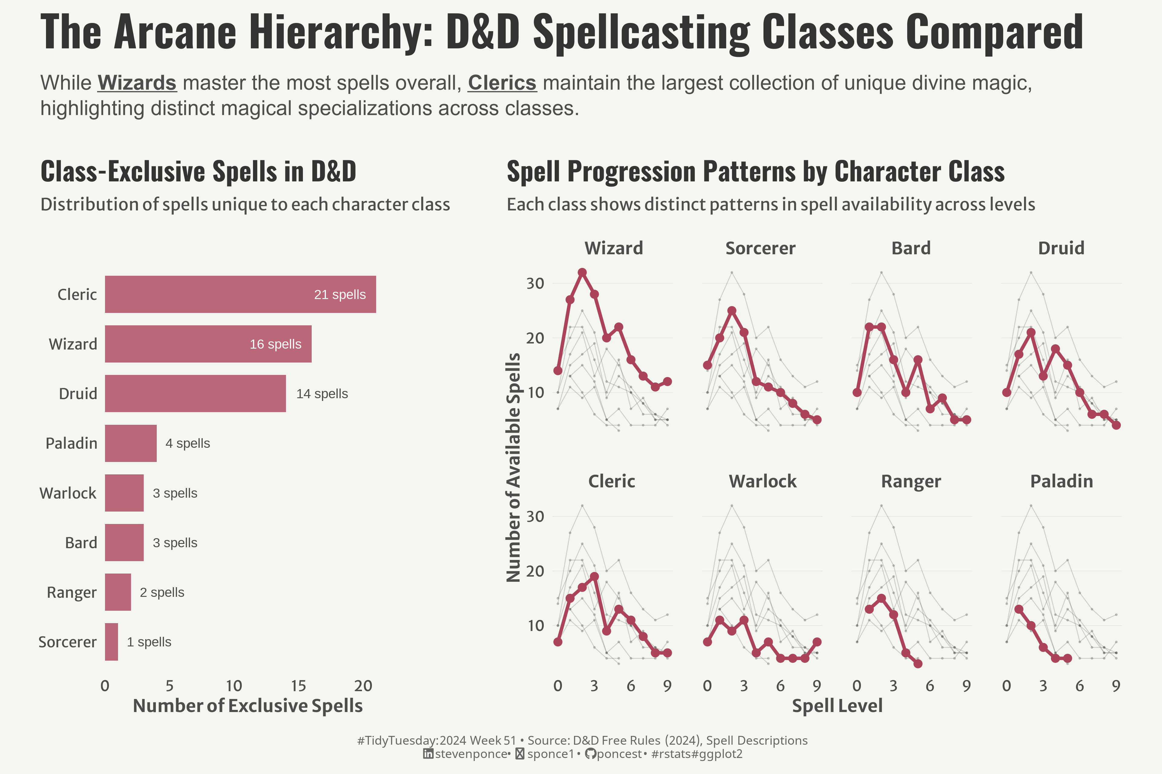
subtitle: "While Wizards master the most spells overall, Clerics maintain the largest collection of unique divine magic, highlighting distinct magical specializations across classes."
description: "An analysis of D&D spellcasting classes examining spell distribution and progression patterns, revealing the unique balance between versatility and specialization among magical practitioners."
author: "Steven Ponce"
date: "2024-12-08"
categories: ["TidyTuesday", "2024"]
tags: [D&D, RPG Games, ggplot2, patchwork, data-viz, spells, fantasy-gaming, class-analysis, tidyverse, spell-progression]
image: "thumbnails/tt_2024_51.png"
format:
html:
toc: true
toc-depth: 5
code-link: true
code-fold: true
code-tools: true
code-summary: "Show code"
editor_options:
chunk_output_type: inline
execute:
freeze: true
cache: true
error: false
message: false
warning: false
eval: true
# filters:
# - social-share
# share:
# permalink: "https://stevenponce.netlify.app/data_visualizations/TidyTuesday/2024/tt_2024_51.html"
# description: "DnD Magic Analysis: Comparing Wizards versatility vs Clerics unique spells. A data story on spellcasting class specializations. #DnD #DataViz #rstats"
# twitter: true
# linkedin: true
# email: true
# facebook: false
# reddit: false
# stumble: false
# tumblr: false
# mastodon: true
# bsky: true
---
{#fig-1}
### <mark> __Steps to Create this Graphic__ </mark>
#### 1. Load Packages & Setup
```{r}
#| label: load
#| warning: false
#| message: false
#| results: "hide"
## 1. LOAD PACKAGES & SETUP ----
suppressPackageStartupMessages({
    pacman::p_load(
    tidyverse,      # Easily Install and Load the 'Tidyverse'
    ggtext,         # Improved Text Rendering Support for 'ggplot2'
    showtext,       # Using Fonts More Easily in R Graphs
    janitor,        # Simple Tools for Examining and Cleaning Dirty Data
    skimr,          # Compact and Flexible Summaries of Data
    scales,         # Scale Functions for Visualization
    glue,           # Interpreted String Literals
    here,           # A Simpler Way to Find Your Files
    camcorder,      # Record Your Plot History
    patchwork,      # The Composer of Plots
    marquee,        # Markdown Parser and Renderer for R Graphics
    gghighlight     # Highlight Lines and Points in 'ggplot2'
    )
})

# Source utility functions
suppressMessages(source(here::here("R/utils/fonts.R")))
source(here::here("R/utils/social_icons.R"))
source(here::here("R/utils/image_utils.R"))
source(here::here("R/themes/base_theme.R"))
```
#### 2. Read in the Data
```{r}
#| label: read
#| include: true
#| eval: true
#| warning: false
# tt <- tidytuesdayR::tt_load(2024, week = 50)
#
# parfumo_data_raw  <- tt$parfumo_data |> clean_names()
#
# tidytuesdayR::readme(tt)
# rm(tt)

# Option 2: Read directly from GitHub
spells_raw <- spells <- readr::read_csv(
  'https://raw.githubusercontent.com/rfordatascience/tidytuesday/main/data/2024/2024-12-17/spells.csv') |>
  clean_names()
```
#### 3. Examine the Data
```{r}
#| label: examine
#| include: true
#| eval: true
#| results: 'hide'
#| warning: false
glimpse(spells_raw)
skim(spells_raw)
```
#### 4. Tidy Data
```{r}
#| label: tidy
#| warning: false
### |- tidy data ----

## Plot 1: Exclusive Spells Data ----
exclusive_df <- spells_raw |>
    # Calculate class availability
    mutate(
        available_to = rowSums(select(spells_raw, bard:wizard))
    ) |>
    # Get exclusive spells
    filter(available_to == 1) |>
    select(bard:wizard) |>
    # Calculate totals
    summarise(across(everything(), sum)) |>
    # Reshape to long format
    pivot_longer(
        everything(),
        names_to = "class",
        values_to = "exclusive_spells"
    ) |>
    # Format and calculate percentages
    mutate(
        class = str_to_title(class),
        total_spells = sum(exclusive_spells),
        pct = exclusive_spells / total_spells,
        label = scales::percent(pct, accuracy = 0.1),
        class = fct_reorder(class, exclusive_spells, .desc = TRUE)
    )

## Plot 2: Progression Data ----
progression_df <- spells_raw |>
    # Initial selection and reshape
    select(level, bard:wizard) |>
    pivot_longer(
        -level,
        names_to = "class",
        values_to = "has_spell"
    ) |>
    # Process available spells
    filter(has_spell) |>
    # Count spells per class and level
    group_by(class, level) |>
    summarise(
        count = n(),
        .groups = "drop"
    ) |>
    # Calculate totals and format
    group_by(class) |>
    mutate(
        total_spells = sum(count)
    ) |>
    ungroup() |>
    # Format and order class factor
    mutate(
        class = str_to_title(class),
        # Order by total spells descending
        class = fct_reorder(class, total_spells, .desc = TRUE)
    )
```
#### 5. Visualization Parameters
```{r}
#| label: params
#| include: true
#| warning: false
### |-  plot aesthetics ----
# Get base colors with custom palette
colors <- get_theme_colors(palette = "#AB4459")


### |-  titles and caption ----
title_text    <- str_glue("The Arcane Hierarchy: D&D Spellcasting Classes Compared")
subtitle_text <- "While **_Wizards_** master the most spells overall, **_Clerics_** maintain the largest collection of unique divine magic, highlighting distinct magical specializations across classes."

# Create caption
caption_text <- create_social_caption(
    tt_year = 2024,
    tt_week = 51,
    source_text = "D&D Free Rules (2024), Spell Descriptions"
)

### |-  fonts ----
setup_fonts()
fonts <- get_font_families()

### |-  plot theme ----

# Start with base theme
base_theme <- create_base_theme(colors)

# Add weekly-specific theme elements
weekly_theme <- extend_weekly_theme(
    base_theme,
    theme(
        # Weekly-specific modifications
        panel.grid.major.x = element_blank(),
        panel.grid.major.y = element_line(color = "gray90", linewidth = 0.2),
        panel.grid.minor   = element_blank(),
        strip.text         = element_textbox(size = rel(0.9),
                                             face = 'bold',
                                             color = colors$text,
                                             hjust = 0.5,
                                             halign = 0.5,
                                             r = unit(3, "pt"),
                                             width = unit(6, "npc"),
                                             padding = margin(2, 0, 2, 0),
                                             margin = margin(3, 3, 3, 3),
                                             fill = "transparent"
        ),
        panel.spacing = unit(1.5, 'lines')
    )
)

# Set theme
theme_set(weekly_theme)
```
#### 6. Plot
```{r}
#| label: plot
#| warning: false
### |-  Plot 1 ----
exclusive_plot <- ggplot(exclusive_df,
                         aes(y = fct_reorder(class, exclusive_spells), x = exclusive_spells)) +
    # Geoms
    geom_bar(stat = "identity",
             fill = colors$palette,
             alpha = 0.8,
             width = 0.75
    ) +
    geom_text(
        aes(label = sprintf("%d spells", exclusive_spells),),
        size = 3.5,
        color = if_else(exclusive_df$exclusive_spells < 15, colors$text, "#fafafa"),
        hjust = if_else(exclusive_df$exclusive_spells < 15, -0.2, 1.2),
    ) +

    # Scales
    scale_x_continuous(
        expand = expansion(mult = c(0, 0.05)),
        breaks = seq(0, 25, by = 5)
    ) +
    scale_y_discrete() +
    coord_cartesian(clip = 'off') +

    # Labs
    labs(
        title = "Class-Exclusive Spells in D&D",
        subtitle = "Distribution of spells unique to each character class",
        x = "Number of Exclusive Spells",
        y = NULL
    ) +

    # Theme
    theme(
        plot.title = element_text(
            family = fonts$title,
            size   = rel(1.4),
            face   = "bold",
            color  = colors$title,
            margin = margin(b = 10)
        ),
        plot.subtitle = element_text(
            family = fonts$text,
            size   = rel(0.9),
            color  = colors$subtitle,
            margin = margin(b = 5)
        ),
        panel.grid.minor = element_blank(),
        panel.grid.major.y = element_blank(),
    )

### |-  Plot 2 ----
progression_plot <- ggplot(progression_df,
                           aes(x = level, y = count, group = class)) +
    # Geoms
    geom_line(size = 0.3, alpha = 0.2) +
    geom_point(size = 1, alpha = 0.2) +
    gghighlight(
        use_direct_label = FALSE,
        unhighlighted_params = list(
            size = 0.3,
            alpha = 0.2,
            color = 'gray20'
        )
    ) +
    geom_line(color = colors$palette, linewidth = 1.2) +
    geom_point(color = colors$palette, size = 2.5) +

    # Scales
    scale_x_continuous(breaks = seq(0, 9, by = 3)) +
    scale_y_continuous(breaks = seq(0, 35, by = 10)) +
    coord_cartesian(clip = 'off') +

    # Labs
    labs(
        title = "Spell Progression Patterns by Character Class",
        subtitle = "Each class shows distinct patterns in spell availability across levels",
        x = "Spell Level",
        y = "Number of Available Spells"
    ) +

    # Facet
    facet_wrap(~class, ncol = 4) +

    # Theme
    theme(
        plot.title = element_text(
            family = fonts$title,
            size   = rel(1.4),
            face   = "bold",
            color  = colors$title,
            margin = margin(b = 10)
        ),
        plot.subtitle = element_text(
            family = fonts$text,
            size   = rel(0.9),
            color  = colors$subtitle,
            margin = margin(b = 15)
        )
    )

### |-  combined plots ----
combined_plot <- (
    exclusive_plot + plot_spacer() + progression_plot +
        plot_layout(widths = c(0.6, 0.02, 1.2))
)

combined_plot <- combined_plot +
    plot_annotation(
        title    = title_text,
        subtitle = subtitle_text,
        caption  = caption_text,
        theme = theme(
            plot.title = element_text(
                family = fonts$title,
                size   = rel(2.3),
                face   = "bold",
                color  = colors$title,
                margin = margin(b = 10)
            ),
            plot.subtitle = element_marquee(
                family = fonts$text,
                lineheight = 1.1,
                width  = 1,
                size   = rel(1.1),
                color  = colors$subtitle,
                margin = margin(b = 5)
            ),
            plot.caption = element_markdown(
                family = fonts$caption,
                lineheight = 1.1,
                size   = rel(0.65),
                color  = colors$caption,
                hjust  = 0.5,
                margin = margin(t = 5)
            ),
            plot.margin = margin(10, 10, 10, 10),
            plot.background = element_rect(fill = colors$background, color = colors$background),
            panel.background = element_rect(fill = colors$background, color = colors$background)
        )
    )
```
#### 7. Save
```{r}
#| label: save
#| warning: false
### |-  plot image ----

save_plot_patchwork(combined_plot, type = "tidytuesday",
                    year = 2024, week = 51, width = 12, height = 8)
```
#### 8. Session Info
::: {.callout-tip collapse="true"}
##### Expand for Session Info
```{r, echo = FALSE}
#| eval: true
#| warning: false
sessionInfo()
```
:::
#### 9. GitHub Repository
::: {.callout-tip collapse="true"}
##### Expand for GitHub Repo
The complete code for this analysis is available in [`tt_2024_51.qmd`](https://github.com/poncest/personal-website/blob/master/data_visualizations/TidyTuesday/2024/tt_2024_51.qmd).
For the full repository, [click here](https://github.com/poncest/personal-website/).
:::
