---
title: "The Paradox of Himalayan Climbing Expeditions"
subtitle: "While larger teams achieve higher success rates, individual climbers face greater risks in smaller teams. Analysis of climbing patterns, team dynamics, and safety implications from 1925 to 2024"
description: "Exploring a compelling paradox in Himalayan mountaineering: while larger teams achieve significantly higher summit success rates (up to 91%), individual climbers actually face greater risks when participating in smaller teams. Through four interconnected visualizations, this analysis reveals historical climbing patterns (1925-2024), geographical distributions across mountain ranges, and the complex relationship between team size and expedition outcomes. The data challenges common assumptions about safety in numbers, showing that although larger teams are more successful, individual safety might be compromised in smaller groups despite their continued appeal to climbers."
author: "Steven Ponce"
date: "2025-01-19"
date-modified: "2025-01-21"
categories: ["TidyTuesday", "2025"]
tags: [
"ggplot2",
"patchwork",
"mountaineering",
"Himalayas",
"time-series",
"data-storytelling",
"exploratory-analysis",
"risk-analysis",
"success-rates",
"pattern-analysis",
"geospatial-data",
"historical-data",
"tidyverse",
"data-wrangling",
"visualization-design"
]
image: "thumbnails/tt_2025_03.png"
format:
html:
toc: true
toc-depth: 5
code-link: true
code-fold: true
code-tools: true
code-summary: "Show code"
editor_options:
chunk_output_type: inline
execute:
freeze: true
cache: true
error: false
message: false
warning: false
eval: true
# filters:
# - social-share
# share:
# permalink: "https://stevenponce.netlify.app/data_visualizations/TidyTuesday/2025/tt_2025_03.html"
# description: "Discover the paradox of Himalayan climbing: while larger teams achieve higher success rates (up to 91%), individual climbers face greater risks in smaller teams. Analysis of 100 years of expedition data reveals fascinating patterns in mountaineering safety and success."
#
# twitter: true
# linkedin: true
# email: true
# facebook: false
# reddit: false
# stumble: false
# tumblr: false
# mastodon: true
# bsky: true
---
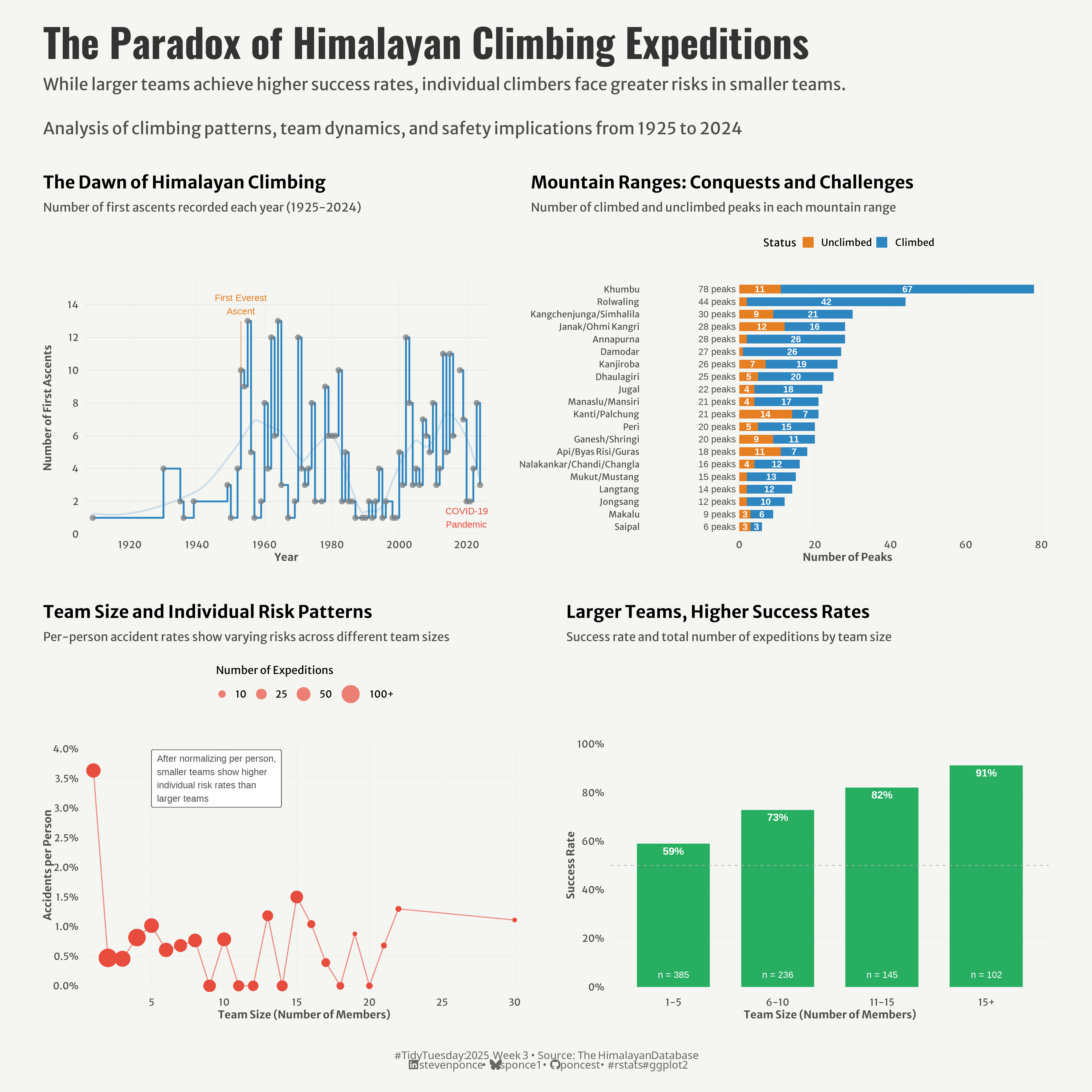{#fig-1}
::: {.callout-note}
## Update (January 21, 2025)
This post has been updated based on valuable feedback from [The Data Digest](https://x.com/DigestData). The changes include:
* Normalizing the accident rates to be per-person rather than per-expedition in the risk analysis plot
* Revising the visualization's subtitle to accurately reflect that individual climbers face greater risks in smaller teams
* Updating the annotation in the risk analysis plot to better explain the relationship between team size and individual risk
* Modifying the color scheme and axis scales in the risk analysis plot to better represent the per-person accident rates
:::
### <mark> **Steps to Create this Graphic** </mark>
#### 1. Load Packages & Setup
```{r}
#| label: load
#| warning: false
#| message: false
#| results: "hide"
## 1. LOAD PACKAGES & SETUP ----
suppressPackageStartupMessages({
if (!require("pacman")) install.packages("pacman")
pacman::p_load(
    tidyverse,      # Easily Install and Load the 'Tidyverse'
    ggtext,         # Improved Text Rendering Support for 'ggplot2'
    showtext,       # Using Fonts More Easily in R Graphs
    janitor,        # Simple Tools for Examining and Cleaning Dirty Data
    skimr,          # Compact and Flexible Summaries of Data
    scales,         # Scale Functions for Visualization
    glue,           # Interpreted String Literals
    here,           # A Simpler Way to Find Your Files
    patchwork       # The Composer of Plots
)

})

# Source utility functions
suppressMessages(source(here::here("R/utils/fonts.R")))
source(here::here("R/utils/social_icons.R"))
source(here::here("R/utils/image_utils.R"))
source(here::here("R/themes/base_theme.R"))
```
#### 2. Read in the Data
```{r}
#| label: read
#| include: true
#| eval: true
#| warning: false
tt <- tidytuesdayR::tt_load(2025, week = 03)

exped_tidy <- tt$exped_tidy |> clean_names()
peaks_tidy <- tt$peaks_tidy |> clean_names()

tidytuesdayR::readme(tt)
rm(tt)
```
#### 3. Examine the Data
```{r}
#| label: examine
#| include: true
#| eval: true
#| results: 'hide'
#| warning: false
glimpse(exped_tidy)
skim(exped_tidy)

glimpse(peaks_tidy)
skim(peaks_tidy)
```
#### 4. Tidy Data
```{r}
#| label: tidy
#| warning: false
# 1. First Ascent Timeline
first_ascents_data <- peaks_tidy |>
  filter(!is.na(pyear)) |>
  group_by(pyear) |>
  summarise(
    first_ascents = n(),
    .groups = "drop"
  ) |>
  # Add flag for special years
  mutate(
    highlight = case_when(
      pyear == 1953 ~ "Everest",
      pyear >= 2020 & pyear <= 2021 ~ "Covid",
      TRUE ~ "Regular"
    )
  )


# 2. Success Rate by Team Size Category
team_success_data <- exped_tidy |>
  filter(totmembers > 0) |>
  mutate(
    team_size = cut(
      totmembers,
      breaks = c(0, 5, 10, 15, Inf),
      labels = c("1-5", "6-10", "11-15", "15+"),
      right = TRUE
    )
  ) |>
  group_by(team_size) |>
  summarise(
    total = n(),
    successes = sum(success1 == TRUE, na.rm = TRUE),
    success_rate = successes / total
  ) |>
  # Create text for labels
  mutate(
    label_position = success_rate,
    success_pct = paste0(round(success_rate * 100), "%"),
    total_label = paste0("n = ", total)
  )

# 3. Distribution of Climbing Status by Mountain Range
climbing_status_data <- peaks_tidy |>
  # Count peaks by range and status
  group_by(himal_factor, pstatus_factor) |>
  summarise(count = n(), .groups = "drop") |>
  # Calculate total peaks per range for sorting
  group_by(himal_factor) |>
  mutate(
    total_peaks = sum(count),
    pct = count / total_peaks,
    # Create labels with count and percentage for larger values
    label = if_else(count >= 3,
      as.character(count),
      ""
    ), # Only show labels for count >= 3
    # Create total peaks label with consistent format
    total_label = paste0(total_peaks, " peaks")
  ) |>
  ungroup() |>
  # Sort by total peaks
  mutate(
    himal_factor = fct_reorder(himal_factor, total_peaks)
  )

# 4. Accidents vs. Expedition Size (updated)
accident_data <- exped_tidy |>
    filter(totmembers > 0, totmembers <= 30) |>
    group_by(totmembers) |>
    summarise(
        total_expeditions = n(),
        total_people = n() * totmembers,                     # updated
        total_deaths = sum(mdeaths + hdeaths, na.rm = TRUE),
        accidents_per_person = total_deaths / total_people,
        .groups = "drop"
    ) |>
    # Filter for more reliable statistics
    filter(total_expeditions >= 5)
```
#### 5. Visualization Parameters
```{r}
#| label: params
#| include: true
#| warning: false
### |-  plot aesthetics ----
# Get base colors with custom palette
colors <- get_theme_colors(palette = c(
    primary   = "#2E86C1",    # Main blue for time series/success
    secondary = "#E67E22",    # Orange for contrasts
    success   = "#27AE60",    # Green for success metrics
    risk      = "#E74C3C",    # Red for risks/accidents
    neutral   = "gray90"      # Background elements
    ))

### |-  titles and caption ----
title_text <- str_glue("The Paradox of Himalayan Climbing Expeditions")

subtitle_text <- str_glue("While larger teams achieve higher success rates, individual climbers face greater risks in smaller teams.\n
                         Analysis of climbing patterns, team dynamics, and safety implications from 1925 to 2024")

# Create caption
caption_text <- create_social_caption(
    tt_year = 2025,
    tt_week = 03,
    source_text = "The Himalayan Database"
)

### |-  fonts ----
setup_fonts()
fonts <- get_font_families()

### |-  plot theme ----

# Start with base theme
base_theme <- create_base_theme(colors)

# Add weekly-specific theme elements
weekly_theme <- extend_weekly_theme(
    base_theme,
    theme(
        # Text styling
        plot.title = element_text(face = "bold", size = rel(1.14), margin = margin(b = 10)),
        plot.subtitle = element_text(color = colors$text, size = rel(0.78), margin = margin(b = 20)),

        # Axis formatting
        axis.title = element_text(color = colors$text, size = 10),
        axis.text = element_text(color = colors$text, size = 9),

        # Legend formatting
        legend.position = "top",
        legend.title = element_text(size = 10),
        legend.text = element_text(size = 9),
        legend.margin = margin(b = 10),

        # Grid customization
        panel.grid.minor = element_blank(),

        # Plot margins
        plot.margin = margin(t = 20, r = 20, b = 20, l = 20),

        # Legend formatting
        legend.box.margin = margin(b = 15),
        legend.spacing = unit(0.2, "cm"),
        legend.box.spacing = unit(0.2, "cm"),
        legend.key.size = unit(0.8, "lines")
    )
)

# Set theme
theme_set(weekly_theme)
```
#### 6. Plot
```{r}
#| label: plot
#| warning: false
### |-  Plot ----

# 1. First Ascent Timeline
p1 <- ggplot(first_ascents_data,
             aes(x = pyear, y = first_ascents)) +
    # Geoms
    geom_hline(
        yintercept = seq(0, 14, 2),
        color = colors$palette["neutral"],
        linewidth = 0.3
    ) +
    geom_step(
        color = colors$palette["primary"],
        linewidth = 0.8
    ) +
    geom_smooth(
        aes(x = pyear, y = first_ascents),
        method = "loess",
        color = alpha(colors$palette["primary"], 0.2),
        se = FALSE,
        linewidth = 0.8,
        span = 0.3
    ) +
    geom_point(
        aes(color = highlight),
        size = 2,
        alpha = 0.7
    ) +
    # Scales
    scale_x_continuous(
        breaks = c(1920, 1940, 1960, 1980, 2000, 2020),
        expand = expansion(mult = c(0.02, 0.02))
    ) +
    scale_y_continuous(
        breaks = seq(0, 14, 2),
        limits = c(0, 14),
        expand = expansion(mult = c(0, 0.1))
    ) +
    scale_color_manual(
        values = c(
            "Everest" = colors$palette["secondary"],
            "Covid" = colors$palette["risk"],
            "Regular" = colors$palette["primary"]
        ),
        guide = "none"
    ) +
    # Annotations
    annotate(
        "text",
        x = 1953,
        y = 14,
        label = "First Everest\nAscent",
        size = 3,
        color = colors$palette["secondary"],
        hjust = 0.5
    ) +
    annotate(
        "segment",
        x = 1953,
        xend = 1953,
        y = 9,
        yend = 13,
        color = colors$palette["secondary"],
        alpha = 0.5,
        linewidth = 0.5
    ) +
    annotate(
        "text",
        x = 2020,
        y = 1,
        label = "COVID-19\nPandemic",
        size = 3,
        color = colors$palette["risk"],
        hjust = 0.5
    ) +
    # Labs
    labs(
        title = "The Dawn of Himalayan Climbing",
        subtitle = "Number of first ascents recorded each year (1925-2024)",
        x = "Year",
        y = "Number of First Ascents"
    ) +
    # Theme
    theme(
        panel.grid.major.y = element_blank(),
        panel.grid.major.x = element_line(color = "gray95")
    )

# 2. Success Rate by Team Size Category
p2 <- ggplot(team_success_data) +
    # Geoms
    geom_col(
        aes(x = team_size, y = success_rate),
        fill = colors$palette["success"],
        width = 0.7
    ) +
    geom_text(
        aes(x = team_size, y = success_rate, label = success_pct),
        nudge_y = -0.03,
        color = "white",
        fontface = "bold",
        size = 3.5
    ) +
    geom_text(
        aes(x = team_size, y = 0, label = total_label),
        nudge_y = 0.05,
        color = "white",
        size = 3
    ) +
    geom_hline(
        yintercept = 0.5,
        linetype = "dashed",
        color = "gray70",
        linewidth = 0.3
    ) +
    # Scales
    scale_y_continuous(
        labels = percent,
        limits = c(0, 1),
        breaks = seq(0, 1, 0.2),
        expand = expansion(mult = c(0.02, 0.02))
    ) +
    # Labs
    labs(
        title = "Larger Teams, Higher Success Rates",
        subtitle = "Success rate and total number of expeditions by team size",
        x = "Team Size (Number of Members)",
        y = "Success Rate"
    ) +
    # Theme
    theme(
        panel.grid.major.x = element_blank(),
        panel.grid.major.y = element_line(color = "gray95")
    )

# 3. Distribution of Climbing Status by Mountain Range
p3 <- ggplot(climbing_status_data,
             aes(x = count,
                 y = himal_factor,
                 fill = pstatus_factor)) +
    # Geoms
    geom_col(
        position = "stack",
        width = 0.7
    ) +
    geom_text(
        aes(label = label),
        position = position_stack(vjust = 0.5),
        color = "white",
        size = 3,
        fontface = "bold"
    ) +
    geom_text(
        data = subset(climbing_status_data, !duplicated(himal_factor)),
        aes(x = -1, label = sprintf("%d peaks", total_peaks)),  # Simplified label
        hjust = 1,
        size = 3,
        color = "gray30"
    ) +
    # Scales
    scale_x_continuous(
        expand = expansion(mult = c(0.3, 0.05)),  # Increased left expansion
        breaks = seq(0, 80, 20)
    ) +
    scale_fill_manual(
        name = "Status",
        breaks = c("Unclimbed", "Climbed"),
        values = setNames(
            c(colors$palette["secondary"], colors$palette["primary"]),
            c("Unclimbed", "Climbed")
        )
    ) +
    # Labs
    labs(
        title = "Mountain Ranges: Conquests and Challenges",
        subtitle = "Number of climbed and unclimbed peaks in each mountain range",
        x = "Number of Peaks",
        y = NULL
    ) +
    # Theme
    theme(
        axis.text.y = element_text(size = 8),
        panel.grid.major.y = element_blank(),
        panel.grid.major.x = element_line(color = "gray95")
    )

# 4. Accidents vs. Expedition Size
# Update p4 plot to use accidents_per_person
p4 <- ggplot(accident_data) +
    # Geoms
    geom_hline(
        yintercept = seq(0, 0.01, 0.002),
        color = "gray95",
        linewidth = 0.3
    ) +
    geom_line(
        aes(x = totmembers, y = accidents_per_person),  # Changed to per-person metric
        color = colors$palette["risk"],
        linewidth = 0.5,
        alpha = 0.6
    ) +
    geom_point(
        aes(x = totmembers, y = accidents_per_person,  # Changed to per-person metric
            size = total_expeditions),
        color = colors$palette["risk"],
        alpha = 0.7,
        stroke = 0
    ) +
    # Update label text to reflect per-person normalization
    geom_label(
        aes(x = 05, y = 0.035,                                                  # updated
            label = "After normalizing per person,\nsmaller teams show higher\nindividual risk rates than\nlarger teams"),
        size = 3,
        color = colors$text,
        #fill = alpha(colors$palette["primary"], 0.01),
        label.size = 0.25,
        label.padding = unit(0.5, "lines"),
        hjust = 0
    ) +
    # Scales
    scale_y_continuous(
        labels = percent_format(),
        limits = c(-0.001, 0.04),
        breaks = seq(0, 0.04, 0.005),
        expand = expansion(mult = c(0, 0.04))
    ) +
    scale_x_continuous(
        breaks = seq(0, 30, 5),
        expand = expansion(mult = c(0.02, 0.02))
    ) +
    scale_size_continuous(
        range = c(2, 8),
        breaks = c(10, 25, 50, 100),
        labels = c("10", "25", "50", "100+"),
        guide = guide_legend(
            title.position = "top",
            override.aes = list(color = colors$palette["risk"], alpha = 0.7)
        )
    ) +
    # Labs
    labs(                                                                       # updated
        title = "Team Size and Individual Risk Patterns",
        subtitle = "Per-person accident rates show varying risks across different team sizes",
        x = "Team Size (Number of Members)",
        y = "Accidents per Person",
        size = "Number of Expeditions"
    ) +
    # Theme
    theme(
        panel.grid.major = element_line(color = "gray95"),
        legend.key = element_blank()
    )

# Combine plots
combined_plot <- (p1 | p3) / (p4 | p2) +
    plot_layout(
        heights = c(1, 1),
        widths = c(1, 1)
    )

combined_plot <- combined_plot +
    # Add title, subtitle, and caption
    plot_annotation(
        title = title_text,
        subtitle = subtitle_text,
        caption = caption_text,
        theme = theme(
            plot.title = element_text(
                size   = rel(2.6),
                family = fonts$title,
                face   = "bold",
                color  = colors$title,
                lineheight = 1.1,
                margin = margin(t = 5, b = 5)
            ),
            plot.subtitle = element_text(
                size   = rel(1.1),
                family = fonts$subtitle,
                color  = colors$subtitle,
                lineheight = 1.1,
                margin = margin(t = 5, b = 15)
            ),
            plot.caption = element_markdown(
                size   = rel(0.7),
                family = fonts$caption,
                color  = colors$caption,
                hjust  = 0.5,
                margin = margin(t = 10)
            )
        )
    ) &
    # Add spacing between plots
    theme(panel.spacing = unit(2, "cm"))
```
#### 7. Save
```{r}
#| label: save
#| warning: false
### |-  plot image ----

save_plot_patchwork(combined_plot, type = "tidytuesday",
          year = 2025, week = 03, width = 14, height = 14)
```
#### 8. Session Info
::: {.callout-tip collapse="true"}
##### Expand for Session Info
```{r, echo = FALSE}
#| eval: true
#| warning: false
sessionInfo()
```
:::
#### 9. GitHub Repository
::: {.callout-tip collapse="true"}
##### Expand for GitHub Repo
The complete code for this analysis is available in [`tt_2025_03.qmd`](https://github.com/poncest/personal-website/blob/master/data_visualizations/TidyTuesday/2025/tt_2025_03.qmd).
For the full repository, [click here](https://github.com/poncest/personal-website/).
:::
#### 10. References
::: {.callout-tip collapse="true"}
##### Expand for References
1. Data Sources:
- TidyTuesday 2025 Week 03: [The History of Himalayan Mountaineering Expeditions](https://github.com/rfordatascience/tidytuesday/tree/main/data/2025/2025-01-21)
:::
