---
title: "Racial and Ethnic Disparities in Reproductive Medicine Research (2010-2023)"
subtitle: "Analysis of 318 studies from high-impact journals examining disparities in reproductive health"
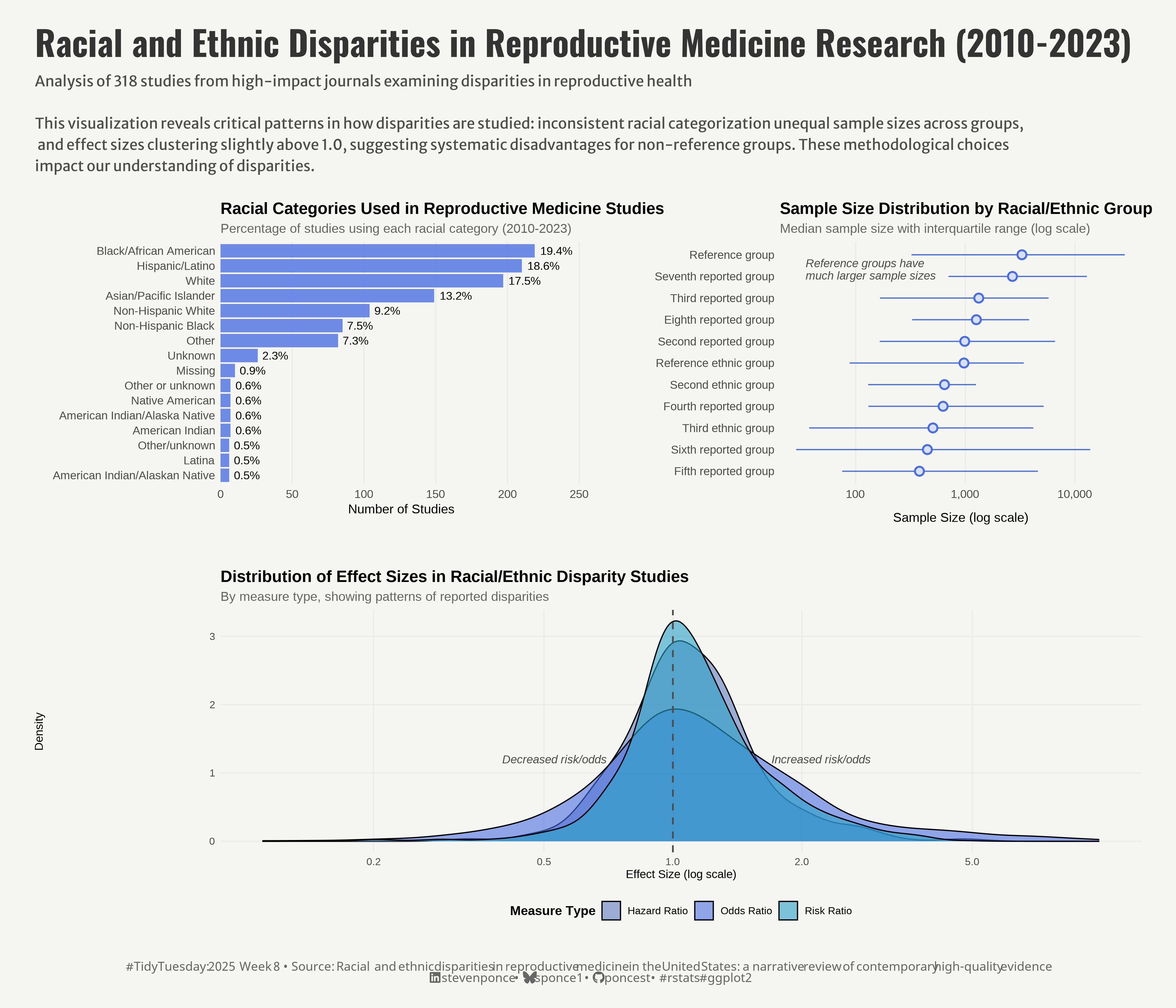
description: "A data visualization analysis examining racial and ethnic disparities in reproductive medicine research. This dashboard reveals critical patterns in how disparities are studied through inconsistent racial categorization, unequal sample sizes across groups, and effect sizes clustering above 1.0, suggesting systematic disadvantages for non-reference groups."
author: "Steven Ponce"
date: "2025-02-24"
categories: ["TidyTuesday", "2025"]
tags: [
"racial disparities", "health equity", "reproductive medicine", "data visualization", "research methodology", "sample size bias", "medical research", "public health", "data analysis", "health disparities", "visualization dashboard", "effect size analysis"
]
image: "thumbnails/tt_2025_08.png"
format:
html:
toc: true
toc-depth: 5
code-link: true
code-fold: true
code-tools: true
code-summary: "Show code"
editor_options:
chunk_output_type: inline
execute:
freeze: true
cache: true
error: false
message: false
warning: false
eval: true
# filters:
# - social-share
# share:
# permalink: "https://stevenponce.netlify.app/data_visualizations/TidyTuesday/2025/tt_2025_08.html"
# description: "Visualizing racial and ethnic disparities in reproductive medicine research (2010-2023): A dashboard revealing inconsistent categorization, sample size disparities, and systematic bias in how reproductive health inequities are studied. #DataViz #HealthEquity #ReproductiveJustice"
#
# twitter: true
# linkedin: true
# email: true
# facebook: false
# reddit: false
# stumble: false
# tumblr: false
# mastodon: true
# bsky: true
---
{#fig-1}
### <mark> **Steps to Create this Graphic** </mark>
#### 1. Load Packages & Setup
```{r}
#| label: load
#| warning: false
#| message: false
#| results: "hide"
## 1. LOAD PACKAGES & SETUP ----
suppressPackageStartupMessages({
if (!require("pacman")) install.packages("pacman")
pacman::p_load(
   tidyverse,      # Easily Install and Load the 'Tidyverse'
    ggtext,         # Improved Text Rendering Support for 'ggplot2'
    showtext,       # Using Fonts More Easily in R Graphs
    janitor,        # Simple Tools for Examining and Cleaning Dirty Data
    skimr,          # Compact and Flexible Summaries of Data
    scales,         # Scale Functions for Visualization
    glue,           # Interpreted String Literals
    here,           # A Simpler Way to Find Your Files
    camcorder,      # Record Your Plot History
    patchwork       # The Composer of Plots # The Composer of Plots # The Composer of Plots
    )
})

### |- figure size ----
gg_record(
    dir    = here::here("temp_plots"),
    device = "png",
    width  =  14,
    height =  12,
    units  = "in",
    dpi    = 320
)

# Source utility functions
suppressMessages(source(here::here("R/utils/fonts.R")))
source(here::here("R/utils/social_icons.R"))
source(here::here("R/utils/image_utils.R"))
source(here::here("R/themes/base_theme.R"))
```
#### 2. Read in the Data
```{r}
#| label: read
#| include: true
#| eval: true
#| warning: false
tt <- tidytuesdayR::tt_load(2025, week = 08)

article_dat <- tt$article_dat |> clean_names()
model_dat <- tt$model_dat |> clean_names()

tidytuesdayR::readme(tt)
rm(tt)
```
#### 3. Examine the Data
```{r}
#| label: examine
#| include: true
#| eval: true
#| results: 'hide'
#| warning: false
glimpse(article_dat)
skim(article_dat)

glimpse(model_dat)
skim(model_dat)
```
#### 4. Tidy Data
```{r}
#| label: tidy
#| warning: false
# P1. Racial Categories -----
racial_categories_data <- article_dat |>
    select(starts_with("race")) |>
    select(matches("race\\d$")) |>  # Select only race categories, not sample sizes
    pivot_longer(everything(), names_to = "category", values_to = "race") |>
    filter(!is.na(race)) |>
    # Standardize category names and combine similar ones
    mutate(race = case_when(
        str_detect(tolower(race), "white.*non.?hispanic|non.?hispanic.*white") ~ "Non-Hispanic White",
        str_detect(tolower(race), "black.*non.?hispanic|non.?hispanic.*black") ~ "Non-Hispanic Black",
        str_detect(tolower(race), "white") ~ "White",
        str_detect(tolower(race), "black|african") ~ "Black/African American",
        str_detect(tolower(race), "hispanic|latino") ~ "Hispanic/Latino",
        str_detect(tolower(race), "asian|pacific") ~ "Asian/Pacific Islander",
        TRUE ~ race
    )) |>
    count(race) |>
    # Filter out very rare categories
    filter(n >= 5) |>
    # Calculate percentage
    mutate(percentage = n/sum(n) * 100) |>
    # Sort by frequency
    arrange(desc(n))


# P2. Sample Size Distribution -----
sample_size_distribution <- article_dat |>
    # Select sample size columns
    select(matches("_ss$")) |>
    # Pivot to long format
    pivot_longer(everything(),
                 names_to = "group",
                 values_to = "size") |>
    # Remove missing values and unreasonable values (-99)
    filter(!is.na(size), size > 0, size != -99) |>
    # Group by racial/ethnic category
    group_by(group) |>
    # Calculate summary statistics
    summarise(
        median_size = median(size),
        mean_size = mean(size),
        q25 = quantile(size, 0.25),
        q75 = quantile(size, 0.75),
        max_size = max(size),
        count = n()
    ) |>
    # Sort by median size for better visualization
    arrange(desc(median_size)) |>
    # Create more readable labels
    mutate(
        group_label = case_when(
            group == "race1_ss" ~ "Reference group",
            group == "race2_ss" ~ "Second reported group",
            group == "race3_ss" ~ "Third reported group",
            group == "race4_ss" ~ "Fourth reported group",
            group == "race5_ss" ~ "Fifth reported group",
            group == "race6_ss" ~ "Sixth reported group",
            group == "race7_ss" ~ "Seventh reported group",
            group == "race8_ss" ~ "Eighth reported group",
            group == "eth1_ss" ~ "Reference ethnic group",
            group == "eth2_ss" ~ "Second ethnic group",
            group == "eth3_ss" ~ "Third ethnic group",
            group == "eth4_ss" ~ "Fourth ethnic group",
            group == "eth5_ss" ~ "Fifth ethnic group",
            group == "eth6_ss" ~ "Sixth ethnic group",
            TRUE ~ group
        )
    ) |>
    # Only include groups with sufficient data
    filter(count >= 5)


# P3. Effect Size Distribution -----
effect_size_data <- model_dat |>
    # Filter for relevant measure types and remove invalid data
    filter(
        measure %in% c("OR", "RR", "HR"),
        point != -99,
        point < 10,
        point > 0.1
    ) |>
    # Add significance indicator
    mutate(
        significance = case_when(
            lower != -99 & upper != -99 & (lower > 1 | upper < 1) ~ "Significant",
            lower != -99 & upper != -99 ~ "Non-significant",
            TRUE ~ "CI Not Reported"
        ),
        # Create a categorized effect size for potential faceting
        effect_category = case_when(
            point < 0.5 ~ "Strong Negative",
            point < 0.8 ~ "Moderate Negative",
            point < 1.0 ~ "Weak Negative",
            point == 1.0 ~ "No Effect",
            point <= 1.25 ~ "Weak Positive",
            point <= 2.0 ~ "Moderate Positive",
            TRUE ~ "Strong Positive"
        ),
        # Rename measure types
        measure = case_when(
            measure == "OR" ~ "Odds Ratio",
            measure == "RR" ~ "Risk Ratio",
            measure == "HR" ~ "Hazard Ratio",
            TRUE ~ measure
        )
    )
```
#### 5. Visualization Parameters
```{r}
#| label: params
#| include: true
#| warning: false
### |-  plot aesthetics ----
# Get base colors with custom palette
colors <- get_theme_colors(
    palette = c(
        "#4A6FE3",
        "#D8E1F3",
        "Odds Ratio" = "#4A6FE3",
        "Risk Ratio" = "#29A2C6",
        "Hazard Ratio" = "#5D7CBA"
    )
)

### |-  titles and caption ----
title_text <- str_glue("Racial and Ethnic Disparities in Reproductive Medicine Research (2010-2023)")

subtitle_text <- str_glue(
    "Analysis of 318 studies from high-impact journals examining disparities in reproductive health\n\n",
    "This visualization reveals critical patterns in how disparities are studied: inconsistent racial categorization unequal sample sizes across groups,\n ",
    "and effect sizes clustering slightly above 1.0, suggesting systematic disadvantages for non-reference groups. These methodological choices \n",
    "impact our understanding of disparities."
)

# Create caption
caption_text <- create_social_caption(
    tt_year = 2025,
    tt_week = 08,
    source_text =  "Racial and ethnic disparities in reproductive medicine in the United States: a narrative review of contemporary high-quality evidence"
)

### |-  fonts ----
setup_fonts()
fonts <- get_font_families()

### |-  plot theme ----

# Start with base theme
base_theme <- create_base_theme(colors)

# Add weekly-specific theme elements
weekly_theme <- extend_weekly_theme(
    base_theme,
    theme(
        # Remove axes
        axis.text = element_blank(),
        axis.title = element_blank(),
        panel.grid = element_blank(),

        # Plot margins
        plot.margin = margin(10, 10, 10, 10),
    )
)

# Set theme
theme_set(weekly_theme)
```
#### 6. Plot
```{r}
#| label: plot
#| warning: false
### |-  Map  ----
# P1. Racial Categories -----
p1 <- ggplot(data = racial_categories_data,
             aes(x = reorder(race, n), y = n)) +
    # Geoms
    geom_bar(stat = "identity",
             fill =  colors$palette[1],
             alpha = 0.8) +
    geom_text(aes(label = sprintf("%.1f%%", percentage)),
              hjust = -0.2,
              size = 3.5) +
    # Scales
    scale_y_continuous(
        expand = expansion(mult = c(0, 0.15)),
        breaks = pretty_breaks()
    ) +
    coord_flip() +
    # Labs
    labs(title = "Racial Categories Used in Reproductive Medicine Studies",
         subtitle = "Percentage of studies using each racial category (2010-2023)",
         x = NULL,
         y = "Number of Studies") +
    # Theme
    theme_minimal() +
    theme(
        plot.title = element_text(face = "bold", size = 14),
        plot.subtitle = element_text(size = 11, color = "gray40"),
        axis.text = element_text(size = 10),
        panel.grid.major.y = element_blank(),
        panel.grid.minor = element_blank(),
        plot.margin = margin(20, 40, 20, 20)
    )


# P2. Sample Size Distribution -----
p2 <- ggplot(data = sample_size_distribution,
             aes(x = reorder(group_label, median_size), y = median_size)) +
    # Geoms
    geom_pointrange(
        aes(ymin = q25, ymax = q75),
        size = 0.7,
        color = colors$palette[1],
        fill =  colors$palette[2],
        shape = 21,
        stroke = 1.2
    ) +
    annotate(
        "text",
        x = 10.8,
        y = 35,
        label = "Reference groups have\nmuch larger sample sizes",
        lineheight = 0.9,
        hjust = 0,
        vjust = 1,
        size = 3.5,
        color = "gray30",
        fontface = "italic"
    ) +
    # Scales
    coord_flip() +
    scale_y_log10(
        labels = label_comma(),
        breaks = c(10, 100, 1000, 10000, 100000)
    ) +
    # Labs
    labs(
        title = "Sample Size Distribution by Racial/Ethnic Group",
        subtitle = "Median sample size with interquartile range (log scale)",
        x = NULL,
        y = "Sample Size (log scale)"
    ) +
    # Theme
    theme_minimal() +
    theme(
        plot.title = element_text(face = "bold", size = 14),
        plot.subtitle = element_text(size = 11, color = "gray40"),
        axis.text = element_text(size = 10),
        axis.title.x = element_text(margin = margin(t = 10)),
        panel.grid.minor = element_blank(),
        panel.grid.major.y = element_blank(),
        plot.margin = margin(20, 20, 20, 20)
    )


# P3. Effect Size Distribution -----
p3 <- ggplot(data = effect_size_data,
             aes(x = point, fill = measure)) +
    # Geoms
    geom_density(alpha = 0.6, adjust = 1.5) +
    geom_vline(                 # Vertical reference line at 1 (no effect)
        xintercept = 1,
        linetype = "dashed",
        color = "gray30",
        size = 0.7
    ) +
    annotate(
        "text",
        x = 0.7,
        y = 1.2,
        label = "Decreased risk/odds",
        hjust = 1,
        size = 3.5,
        fontface = "italic",
        color = "gray30"
    ) +
    annotate(
        "text",
        x = 1.7,
        y = 1.2,
        label = "Increased risk/odds",
        hjust = 0,
        size = 3.5,
        fontface = "italic",
        color = "gray30"
    ) +
    # Scales
    scale_fill_manual(
        values =  colors$palette
    ) +
    scale_x_log10(
        breaks = c(0.2, 0.5, 1, 2, 5),
        labels = c("0.2", "0.5", "1.0", "2.0", "5.0")
    ) +
    # Labs
    labs(
        title = "Distribution of Effect Sizes in Racial/Ethnic Disparity Studies",
        subtitle = "By measure type, showing patterns of reported disparities",
        x = "Effect Size (log scale)",
        y = "Density",
        fill = "Measure Type"
    ) +
    # Theme
    theme_minimal() +
    theme(
        plot.title = element_text(face = "bold", size = 14),
        plot.subtitle = element_text(size = 11, color = "gray40"),
        axis.title = element_text(size = 10),
        legend.position = "bottom",
        legend.title = element_text(face = "bold"),
        panel.grid.minor = element_blank(),
        plot.margin = margin(20, 20, 20, 20)
    )

# Combined Plot -----
combined_plot <- (p1 + p2) / p3 +
    plot_layout(heights = c(1, 1)) +
    plot_annotation(
        title = title_text,
        subtitle = subtitle_text,
        caption = caption_text,
        theme = theme(
            plot.title = element_text(
                size   = rel(2.1),
                family = fonts$title,
                face   = "bold",
                color  = colors$title,
                lineheight = 1.1,
                margin = margin(t = 5, b = 5)
            ),
            plot.subtitle = element_text(
                size   = rel(0.9),
                family = fonts$subtitle,
                color  = colors$subtitle,
                lineheight = 1.2,
                margin = margin(t = 5, b = 5)
            ),
            plot.caption = element_markdown(
                size   = rel(0.75),
                family = fonts$caption,
                color  = colors$caption,
                hjust  = 0.5,
                margin = margin(t = 10)
            ),
            plot.margin = margin(t = 20, r = 10, b = 20, l = 10),
        )
    )
```
#### 7. Save
```{r}
#| label: save
#| warning: false
### |-  plot image ----
save_plot_patchwork(
  plot = combined_plot,
  type = "tidytuesday",
  year = 2025,
  week = 8,
  width = 14,
  height = 12
)
```
#### 8. Session Info
::: {.callout-tip collapse="true"}
##### Expand for Session Info
```{r, echo = FALSE}
#| eval: true
#| warning: false
sessionInfo()
```
:::
#### 9. GitHub Repository
::: {.callout-tip collapse="true"}
##### Expand for GitHub Repo
The complete code for this analysis is available in [`tt_2025_08.qmd`](https://github.com/poncest/personal-website/blob/master/data_visualizations/TidyTuesday/2025/tt_2025_08.qmd).
For the full repository, [click here](https://github.com/poncest/personal-website/).
:::
#### 10. References
::: {.callout-tip collapse="true"}
##### Expand for References
1. Data Sources:
- TidyTuesday 2025 Week 08]: [Academic Literature on Racial and Ethnic Disparities in Reproductive Medicine in the US](https://github.com/rfordatascience/tidytuesday/blob/main/data/2025/2025-02-25)
:::
