---
title: "Growth Form Patterns Across Palm Subfamilies"
subtitle: "Relationship between taxonomic classification and physical growth characteristics"
description: "Exploring growth patterns and morphological diversity across palm tree subfamilies using the PalmTraits 1.0 database, revealing how evolutionary history shapes physical characteristics."
author: "Steven Ponce"
date: "2025-03-17"
categories: ["TidyTuesday", "2025"]
tags: [
"alluvial diagram", "palm trees", "botanical diversity", "taxonomy", "morphology", "evolutionary biology", "growth forms", "ggalluvial", "plant traits", "biodiversity"
]
image: "thumbnails/tt_2025_11.png"
format:
html:
toc: true
toc-depth: 5
code-link: true
code-fold: true
code-tools: true
code-summary: "Show code"
editor_options:
chunk_output_type: inline
execute:
freeze: true
cache: true
error: false
message: false
warning: false
eval: true
# filters:
# - social-share
# share:
# permalink: "https://stevenponce.netlify.app/data_visualizations/TidyTuesday/2025/tt_2025_11.html"
# description: "Exploring palm tree evolution through growth patterns: this #TidyTuesday visualization reveals how different palm subfamilies have developed distinctive growth strategies and morphological traits."
#
# twitter: true
# linkedin: true
# email: true
# facebook: false
# reddit: false
# stumble: false
# tumblr: false
# mastodon: true
# bsky: true
---
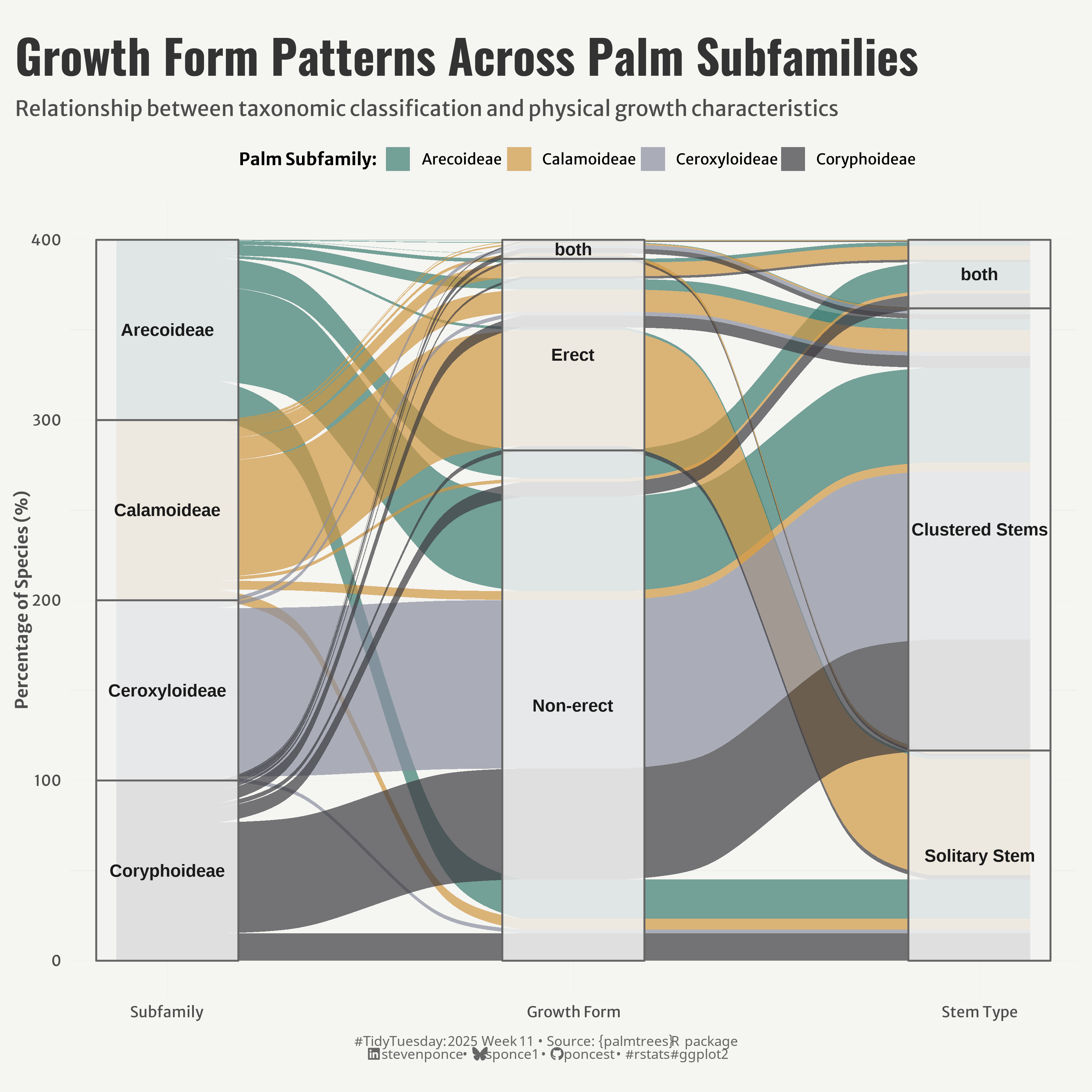{#fig-1}
### <mark> **Steps to Create this Graphic** </mark>
#### 1. Load Packages & Setup
```{r}
#| label: load
#| warning: false
#| message: false
#| results: "hide"
## 1. LOAD PACKAGES & SETUP ----
suppressPackageStartupMessages({
if (!require("pacman")) install.packages("pacman")
pacman::p_load(
    tidyverse,      # Easily Install and Load the 'Tidyverse'
    ggtext,         # Improved Text Rendering Support for 'ggplot2'
    showtext,       # Using Fonts More Easily in R Graphs
    janitor,        # Simple Tools for Examining and Cleaning Dirty Data
    skimr,          # Compact and Flexible Summaries of Data
    scales,         # Scale Functions for Visualization
    glue,           # Interpreted String Literals
    here,           # A Simpler Way to Find Your Files
    camcorder,      # Record Your Plot History
    ggalluvial,     # Alluvial Plots in 'ggplot2'
    MetBrewer      # Color Palettes Inspired by Works at the Metropolitan Museum of Art
    )
})

### |- figure size ----
gg_record(
    dir    = here::here("temp_plots"),
    device = "png",
    width  =  10,
    height =  10,
    units  = "in",
    dpi    = 320
)

# Source utility functions
suppressMessages(source(here::here("R/utils/fonts.R")))
source(here::here("R/utils/social_icons.R"))
source(here::here("R/utils/image_utils.R"))
source(here::here("R/themes/base_theme.R"))
```
#### 2. Read in the Data
```{r}
#| label: read
#| include: true
#| eval: true
#| warning: false
tt <- tidytuesdayR::tt_load(2025, week = 11)

palmtrees_raw <- tt$palmtrees |> clean_names()

tidytuesdayR::readme(tt)
rm(tt)
```
#### 3. Examine the Data
```{r}
#| label: examine
#| include: true
#| eval: true
#| results: 'hide'
#| warning: false
glimpse(palmtrees_raw)
skim(palmtrees_raw)
```
#### 4. Tidy Data
```{r}
#| label: tidy
#| warning: false
### |-  tidy data ----
growth_form_data <- palmtrees_raw |>
    filter(!is.na(erect), !is.na(stem_solitary), !is.na(palm_subfamily)) |>
    count(palm_subfamily, erect, stem_solitary) |>
    group_by(palm_subfamily) |>
    filter(sum(n) > 20) |>
    mutate(percentage = n / sum(n) * 100) |>
    ungroup() |>
    mutate(
        erect_label = case_when(
            erect == "erect" ~ "Erect",
            erect == "non-erect" ~ "Non-erect",
            TRUE ~ as.character(erect)
        ),
        stem_solitary_label = case_when(
            stem_solitary == "solitary" ~ "Solitary Stem",
            stem_solitary == "non-solitary" ~ "Clustered Stems",
            TRUE ~ as.character(stem_solitary)
        ),
        palm_subfamily = str_to_title(palm_subfamily)
    )
```
#### 5. Visualization Parameters
```{r}
#| label: params
#| include: true
#| warning: false
### |-  plot aesthetics ----
colors <- get_theme_colors(
    palette = MetBrewer::met.brewer(
        name = "Kandinsky",
        n = 4,
        type = 'discrete')
)

### |-  titles and caption ----
title_text <- str_glue("Growth Form Patterns Across Palm Subfamilies")
subtitle_text <- str_glue("Relationship between taxonomic classification and physical growth characteristics")

# Create caption
caption_text <- create_social_caption(
    tt_year = 2025,
    tt_week = 11,
    source_text =  "{palmtrees} R package"
)

### |-  fonts ----
setup_fonts()
fonts <- get_font_families()

### |-  plot theme ----

# Start with base theme
base_theme <- create_base_theme(colors)

# Add weekly-specific theme elements
weekly_theme <- extend_weekly_theme(
    base_theme,
    theme(
        # Text styling
        plot.title = element_text(face = "bold", family = fonts$title, size = rel(1.14), margin = margin(b = 10)),
        plot.subtitle = element_text(family = fonts$subtitle, color = colors$text, size = rel(0.78), margin = margin(b = 20)),

        # Axis elements
        axis.title = element_text(color = colors$text, face = "bold", size = rel(0.8)),
        axis.text = element_text(color = colors$text, size = rel(0.7)),

        # Grid elements
        panel.grid.minor = element_line(color = "gray80", linewidth = 0.05),
        panel.grid.major = element_line(color = "gray80", linewidth = 0.02),

        # Legend elements
        legend.position = "top",
        legend.direction = "horizontal",
        legend.title = element_text(family = fonts$text, size = rel(0.8), face = "bold"),
        legend.text = element_text(family = fonts$text, size = rel(0.7)),

        # Plot margins
        plot.margin = margin(t = 10, r = 10, b = 10, l = 10),
    )
)

# Set theme
theme_set(weekly_theme)
```
#### 6. Plot
```{r}
#| label: plot
#| warning: false
### |-  Plot  ----
p <- ggplot(
    data = growth_form_data,
    aes(
        y = percentage,
        axis1 = palm_subfamily,
        axis2 = erect_label,
        axis3 = stem_solitary_label
        )
    ) +

    # Geoms                                   # flow appearance
    geom_alluvium(aes(fill = palm_subfamily),
                  width = 0.25,
                  alpha = 0.7,
                  knot.pos = 0.3
    ) +
    geom_stratum(                             # strata appearance
        width = 0.35,
        fill = "gray95",
        color = "gray40",
        size = 0.6,
        alpha = 0.85
    ) +
    geom_text(
        stat = "stratum",
        aes(label = after_stat(stratum)),
        size = 4,
        fontface = "bold",
        color = "gray10"
    ) +

    # Scales
    scale_x_discrete(
        limits = c("Subfamily", "Growth Form", "Stem Type"),
        expand = c(0.08, 0.08)
    ) +
    scale_fill_manual(values = colors$palette) +
    coord_cartesian(clip = 'off') +

    # Labs
    labs(
        title = title_text,
        subtitle = subtitle_text,
        caption = caption_text,
        y = "Percentage of Species (%)",
        x = NULL
    ) +

    # Legend
    guides(
        fill = guide_legend(title = "Palm Subfamily: ", nrow = 1)
    ) +

    # Theme
    theme(
        plot.title = element_text(
            size = rel(2.2),
            family = fonts$title,
            face = "bold",
            color = colors$title,
            lineheight = 1.1,
            margin = margin(t = 5, b = 5)
        ),
        plot.subtitle = element_text(
            size = rel(1.0),
            family = fonts$subtitle,
            color = colors$subtitle,
            lineheight = 1.2,
            margin = margin(t = 5, b = 10)
        ),
        plot.caption = element_markdown(
            size   = rel(0.65),
            family = fonts$caption,
            color  = colors$caption,
            hjust  = 0.5,
            margin = margin(t = 10)
        ),
        plot.margin = margin(t = 20, r = 10, b = 20, l = 10),
    )
```
#### 7. Save
```{r}
#| label: save
#| warning: false
### |-  plot image ----
save_plot_patchwork(
  plot = p,
  type = "tidytuesday",
  year = 2025,
  week = 11,
  width = 10,
  height = 10
)
```
#### 8. Session Info
::: {.callout-tip collapse="true"}
##### Expand for Session Info
```{r, echo = FALSE}
#| eval: true
#| warning: false
sessionInfo()
```
:::
#### 9. GitHub Repository
::: {.callout-tip collapse="true"}
##### Expand for GitHub Repo
The complete code for this analysis is available in [`tt_2025_11.qmd`](https://github.com/poncest/personal-website/blob/master/data_visualizations/TidyTuesday/2025/tt_2025_11.qmd).
For the full repository, [click here](https://github.com/poncest/personal-website/).
:::
#### 10. References
::: {.callout-tip collapse="true"}
##### Expand for References
1. Data Sources:
- TidyTuesday 2025 Week 11: [Palm Trees](https://github.com/rfordatascience/tidytuesday/blob/main/data/2025/2025-03-18)
:::
