---
title: "Project Gutenberg: Language Patterns in Author Longevity"
subtitle: "Comparing lifespans of English vs non-English authors across centuries"
description: "Exploring author longevity patterns in Project Gutenberg's digital library through advanced data visualization. This TidyTuesday analysis reveals how English-language publishing dominated the 19th century while uncovering surprising differences in author lifespans across languages and time periods using beeswarm plots and statistical analysis."
author: "Steven Ponce"
date: "2025-06-03"
categories: ["TidyTuesday", "2025"]
tags: [
"beeswarm-plot", "statistical-visualization", "literary-analysis",
"digital-humanities", "ggbeeswarm", "author-demographics",
"historical-data", "publishing-patterns", "multilingual-analysis"
]
image: "thumbnails/tt_2025_22.png"
format:
html:
toc: true
toc-depth: 5
code-link: true
code-fold: true
code-tools: true
code-summary: "Show code"
editor_options:
chunk_output_type: inline
execute:
freeze: true
cache: true
error: false
message: false
warning: false
eval: true
---
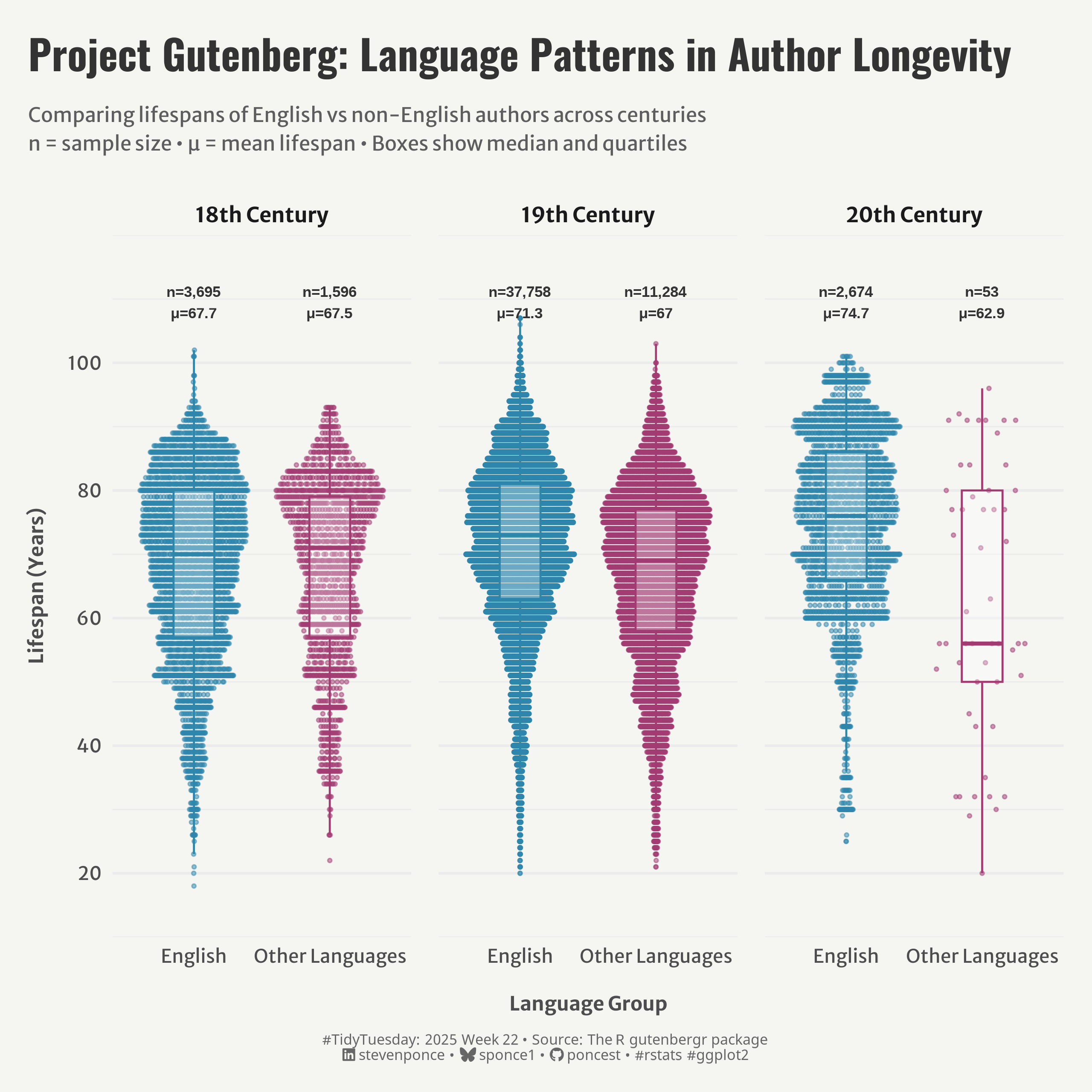{#fig-1}
### <mark> **Steps to Create this Graphic** </mark>
#### 1. Load Packages & Setup
```{r}
#| label: load
#| warning: false
#| message: false
#| results: "hide"

## 1. LOAD PACKAGES & SETUP ----
suppressPackageStartupMessages({
if (!require("pacman")) install.packages("pacman")
pacman::p_load(
  tidyverse,     # Easily Install and Load the 'Tidyverse'
  ggtext,        # Improved Text Rendering Support for 'ggplot2'
  showtext,      # Using Fonts More Easily in R Graphs
  janitor,       # Simple Tools for Examining and Cleaning Dirty Data
  scales,        # Scale Functions for Visualization
  glue,          # Interpreted String Literals
  ggbeeswarm     # Categorical Scatter (Violin Point) Plots
  )
})

### |- figure size ----
camcorder::gg_record(
  dir    = here::here("temp_plots"),
  device = "png",
  width  =  8,
  height =  8,
  units  = "in",
  dpi    = 320
)

# Source utility functions
suppressMessages(source(here::here("R/utils/fonts.R")))
source(here::here("R/utils/social_icons.R"))
source(here::here("R/utils/image_utils.R"))
source(here::here("R/themes/base_theme.R"))
```
#### 2. Read in the Data
```{r}
#| label: read
#| include: true
#| eval: true
#| warning: false

tt <- tidytuesdayR::tt_load(2025, week = 22)

authors_raw <- tt$gutenberg_authors |> clean_names()
languages_raw <- tt$gutenberg_languages |> clean_names()
metadata_raw <- tt$gutenberg_metadata |> clean_names()
subjects_raw <- tt$gutenberg_subjects |> clean_names()

tidytuesdayR::readme(tt)
rm(tt)
```
#### 3. Examine the Data
```{r}
#| label: examine
#| include: true
#| eval: true
#| results: 'hide'
#| warning: false

glimpse(authors_raw)
skimr::skim(authors_raw)
```
#### 4. Tidy Data
```{r}
#| label: tidy
#| warning: false

### |-  tidy data ----
# Preprocessing
authors_clean <- authors_raw |>
  mutate(
    lifespan = deathdate - birthdate,
    birth_century = case_when(
      birthdate >= 1800 & birthdate < 1900 ~ "19th Century",
      birthdate >= 1700 & birthdate < 1800 ~ "18th Century",
      birthdate >= 1900 & birthdate < 2000 ~ "20th Century",
      birthdate < 1700 ~ "Pre-18th Century",
      TRUE ~ "Unknown"
    )
  )

# Join datasets
full_data <- metadata_raw |>
  left_join(languages_raw, by = "gutenberg_id") |>
  left_join(authors_clean, by = "gutenberg_author_id")

# Beeswarm data
beeswarm_data <- full_data |>
  select(lifespan, birth_century, language.x, author.x) |>
  rename(language = language.x, author = author.x) |>
  filter(
    !is.na(lifespan), lifespan > 0, lifespan < 120,
    !is.na(birth_century), birth_century != "Unknown"
  ) |>
  mutate(
    highlight = ifelse(language == "en", "English", "Other Languages"),
    birth_century = factor(birth_century,
      levels = c(
        "Pre-18th Century", "18th Century",
        "19th Century", "20th Century"
      )
    )
  )

# Stats for annotations
detailed_stats <- beeswarm_data |>
  filter(birth_century %in% c("18th Century", "19th Century", "20th Century")) |>
  group_by(birth_century, highlight) |>
  summarise(
    median_lifespan = median(lifespan, na.rm = TRUE),
    count = n(),
    mean_lifespan = round(mean(lifespan, na.rm = TRUE), 1),
    .groups = "drop"
  )
```
#### 5. Visualization Parameters
```{r}
#| label: params
#| include: true
#| warning: false

### |-  plot aesthetics ----
colors <- get_theme_colors(
    palette = c(
        "English" = "#2E86AB", "Other Languages" = "#A23B72"
    )
)

### |-  titles and caption ----
title_text <- str_glue("Project Gutenberg: Language Patterns in Author Longevity")

subtitle_text <- str_glue("Comparing lifespans of English vs non-English authors across centuries\n",
                          "n = sample size • μ = mean lifespan • Boxes show median and quartiles")

caption_text <- create_social_caption(
  tt_year = 2025,
  tt_week = 22,
  source_text =  "The R gutenbergr package"
)

### |-  fonts ----
setup_fonts()
fonts <- get_font_families()

### |-  plot theme ----

# Start with base theme
base_theme <- create_base_theme(colors)

# Add weekly-specific theme elements
weekly_theme <- extend_weekly_theme(
  base_theme,
  theme(
    # Axis elements
    axis.text = element_text(color = colors$text, size = rel(0.7)),
    axis.title.x = element_text(color = colors$text, face = "bold", size = rel(0.8), margin = margin(t = 15)),
    axis.title.y = element_text(color = colors$text, face = "bold", size = rel(0.8), margin = margin(r = 10)),

    # Grid elements
    panel.grid.minor.x = element_line(color = 'gray50', linewidth = 0.05),
    panel.grid.major.x = element_blank(), #element_line(color = 'gray50', linewidth = 0.1),

    # Legend elements
    legend.position = "plot",
    legend.title = element_text(family = fonts$tsubtitle, color = colors$text, size = rel(0.8), face = "bold"),
    legend.text = element_text(family = fonts$tsubtitle, color = colors$text, size = rel(0.7)),

    # Plot margins
    plot.margin = margin(t = 15, r = 15, b = 15, l = 15),
  )
)

# Set theme
theme_set(weekly_theme)
```
#### 6. Plot
```{r}
#| label: plot
#| warning: false

# Final plot -----
p <- beeswarm_data |>
    filter(birth_century %in% c("18th Century", "19th Century", "20th Century")) |>
    ggplot(aes(x = highlight, y = lifespan, color = highlight)) +
    # Geoms
    geom_quasirandom(alpha = 0.5, size = 0.7) +
    geom_boxplot(alpha = 0.3, outlier.shape = NA, width = 0.3) +
    geom_text(data = detailed_stats,
              aes(x = highlight, y = 112,
                  label = paste0("n=", scales::comma(count), "\nμ=", mean_lifespan)),
              color = "gray20", size = 2.8, inherit.aes = FALSE,
              vjust = 1, fontface = "bold") +
    # Scales
    scale_color_manual(values = colors$palette) +
    scale_y_continuous(breaks = seq(20, 100, 20), limits = c(15, 115)) +
    # Facets
    facet_wrap(~birth_century, scales = "free_x") +
    # Labs
    labs(
        title = title_text,
        subtitle = subtitle_text,
        caption = caption_text,
        x = "Language Group",
        y = "Lifespan (Years)",
    ) +
  # Theme
  theme(
    plot.title = element_text(
      size = rel(1.55),
      family = fonts$title,
      face = "bold",
      color = colors$title,
      lineheight = 1.1,
      margin = margin(t = 5, b = 10)
    ),
    plot.subtitle = element_text(
      size = rel(0.75),
      family = fonts$subtitle,
      color = alpha(colors$subtitle, 0.9),
      lineheight = 1.2,
      margin = margin(t = 5, b = 20)
    ),
    plot.caption = element_markdown(
      size = rel(0.55),
      family = fonts$caption,
      color = colors$caption,
      hjust = 0.5,
      margin = margin(t = 10)
    ),
    strip.text = element_text(size = rel(0.78), face = "bold"),
    panel.spacing = unit(1, "lines"),
  )
```
#### 7. Save
```{r}
#| label: save
#| warning: false

### |-  plot image ----
save_plot(
  plot = p,
  type = "tidytuesday",
  year = 2025,
  week = 22,
  width = 8,
  height = 8
)
```
#### 8. Session Info
::: {.callout-tip collapse="true"}
##### Expand for Session Info
```{r, echo = FALSE}
#| eval: true
#| warning: false
sessionInfo()
```
:::
#### 9. GitHub Repository
::: {.callout-tip collapse="true"}
##### Expand for GitHub Repo
The complete code for this analysis is available in [`tt_2025_22.qmd`](https://github.com/poncest/personal-website/blob/master/data_visualizations/TidyTuesday/2025/tt_2025_22.qmd).
For the full repository, [click here](https://github.com/poncest/personal-website/).
:::
#### 10. References
::: {.callout-tip collapse="true"}
##### Expand for References
1. Data Sources:
- TidyTuesday 2025 Week 22: [DProject Gutenberg)](https://github.com/rfordatascience/tidytuesday/blob/main/data/2025/2025-06-03)
:::
