---
title: "From Macarena to Bad Bunny: Latin Music's Billboard Evolution"
subtitle: "Five cultural waves that transformed American popular music (1995-2022)"
description: "Analyzing Latin music's Billboard Hot 100 evolution from 1995-2022 through data visualization. This TidyTuesday project tracks five cultural waves that transformed American charts, from Macarena's dance revolution to Bad Bunny's streaming dominance, using R and ggplot2 to reveal Latin music's path from crossover novelty to mainstream success."
author: "Steven Ponce"
date: "2025-08-25"
categories: ["TidyTuesday", "2025"]
tags: [
"billboard",
"latin-music",
"music-analysis",
"cultural-trends",
"chart-analysis",
"ggplot2",
"faceted-charts",
"timeline-visualization",
"music-industry",
"cultural-impact",
"streaming-era",
"reggaeton",
"data-storytelling"
]
image: "thumbnails/tt_2025_34.png"
format:
html:
toc: true
toc-depth: 5
code-link: true
code-fold: true
code-tools: true
code-summary: "Show code"
editor_options:
chunk_output_type: inline
execute:
freeze: true
cache: true
error: false
message: false
warning: false
eval: true
---
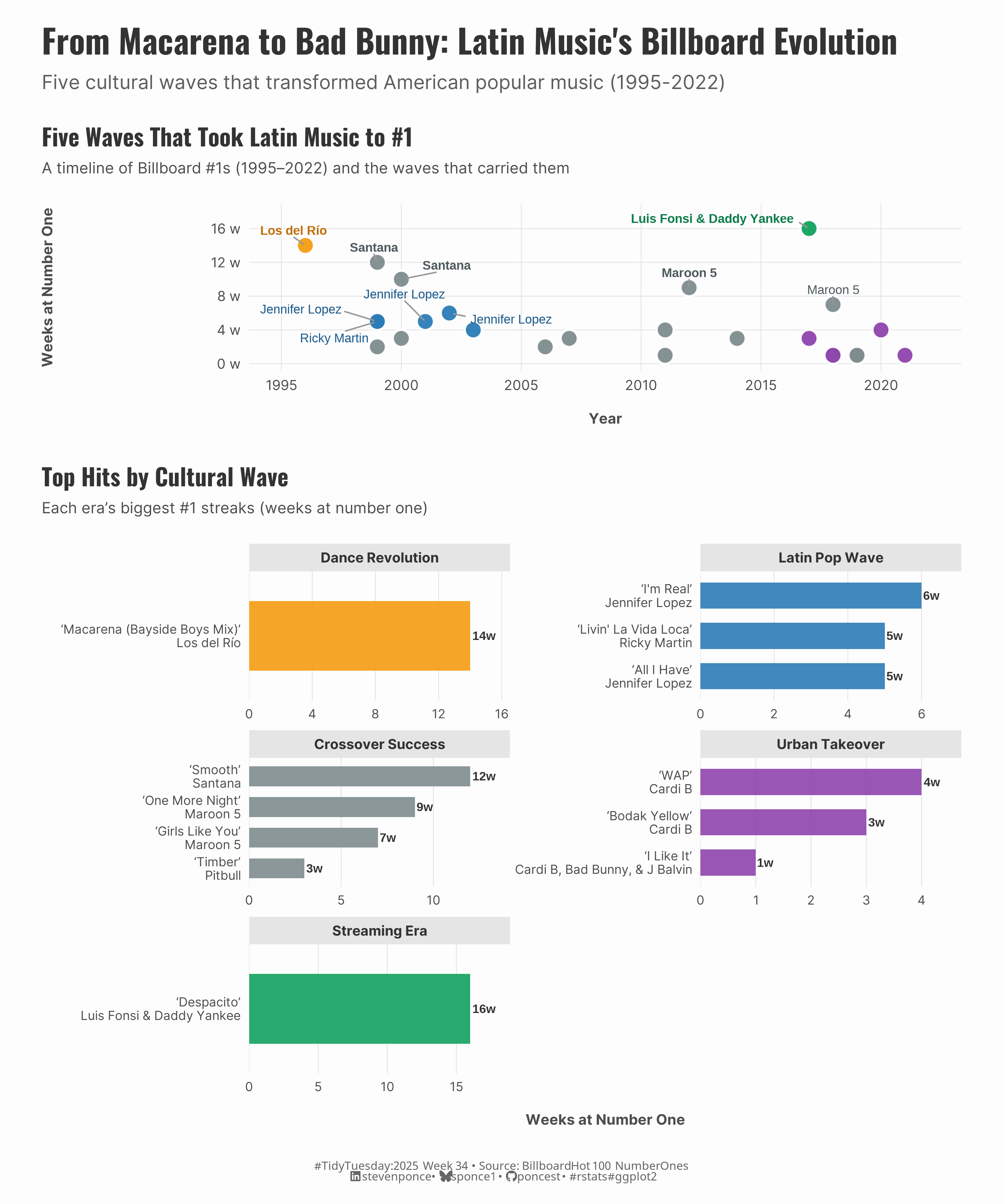{#fig-1}
### <mark> **Steps to Create this Graphic** </mark>
#### 1. Load Packages & Setup
```{r}
#| label: load
#| warning: false
#| message: false
#| results: "hide"

## 1. LOAD PACKAGES & SETUP ----
suppressPackageStartupMessages({
if (!require("pacman")) install.packages("pacman")
pacman::p_load(
    tidyverse,   # Easily Install and Load the 'Tidyverse'
    ggtext,      # Improved Text Rendering Support for 'ggplot2'
    showtext,    # Using Fonts More Easily in R Graphs
    janitor,     # Simple Tools for Examining and Cleaning Dirty Data
    scales,      # Scale Functions for Visualization
    glue,        # Interpreted String Literals,
    ggrepel,     # Automatically Position Non-Overlapping Text Labels with 'ggplot2'
    patchwork    # The Composer of Plots
  )})

### |- figure size ----
camcorder::gg_record(
  dir    = here::here("temp_plots"),
  device = "png",
  width  = 10,
  height = 12,
  units  = "in",
  dpi    = 300
)

# Source utility functions
suppressMessages(source(here::here("R/utils/fonts.R")))
source(here::here("R/utils/social_icons.R"))
source(here::here("R/utils/image_utils.R"))
source(here::here("R/themes/base_theme.R"))
```
#### 2. Read in the Data
```{r}
#| label: read
#| include: true
#| eval: true
#| warning: false

tt <- tidytuesdayR::tt_load(2025, week = 34)

billboard <- tt$billboard |> clean_names()
topics <- tt$topics |> clean_names()

tidytuesdayR::readme(tt)
rm(tt)
```
#### 3. Examine the Data
```{r}
#| label: examine
#| include: true
#| eval: true
#| results: 'hide'
#| warning: false

glimpse(billboard)
glimpse(topics)
```
#### 4. Tidy Data
```{r}
#| label: tidy
#| warning: false

billboard_latin_clean <- billboard |>
  mutate(
    date = if (inherits(date, "Date")) date else as.Date(date),
    year = year(date),
    is_latin_country = artist_place_of_origin %in% c(
      "Mexico", "Puerto Rico", "Colombia", "Argentina", "Spain",
      "Cuba", "Dominican Republic", "Venezuela", "Peru", "Chile",
      "Ecuador", "Guatemala", "Costa Rica", "Panama", "Brazil"
    ),
    is_latin_artist = case_when(
      str_detect(tolower(artist), paste(c(
        "shakira", "ricky martin", "jennifer lopez|j\\.?lo", "marc anthony",
        "enrique iglesias", "luis fonsi", "daddy yankee", "ozuna|bad bunny|j balvin|maluma",
        "camila cabello|pitbull", "santana", "selena", "los del rio",
        "cardi b", "maroon 5"
      ), collapse = "|")) ~ TRUE,
      is_latin_country ~ TRUE,
      TRUE ~ FALSE
    ),
    spanish_language = case_when(
      str_detect(tolower(song), paste(c(
        "despacito", "macarena", "la vida loca", "gasolina", "danza kuduro", "baila", "amor", "corazón"
      ), collapse = "|")) ~ TRUE,
      foreign_language == 1 & is_latin_artist ~ TRUE,
      TRUE ~ FALSE
    )
  ) |>
  filter(is_latin_artist, !is.na(year), !is.na(weeks_at_number_one)) |>
  mutate(
    song_clean = case_when(
      str_detect(artist, "Los del Río") ~ "Macarena (Bayside Boys Mix)",
      str_detect(artist, "Santana ft. Rob Thomas") ~ "Smooth",
      str_detect(artist, "Santana") & !str_detect(artist, "ft.") ~ "Smooth",
      str_detect(artist, "Maroon 5 ft. Cardi B") ~ "Girls Like You",
      str_detect(artist, "Maroon 5") & year == 2012 ~ "One More Night",
      str_detect(artist, "Maroon 5") ~ "Girls Like You",
      str_detect(artist, "Pitbull ft. Kesha") ~ "Timber",
      str_detect(artist, "Jennifer Lopez ft. Ja Rule & Caddillac Tah") ~ "I'm Real",
      str_detect(artist, "Ricky Martin") ~ "Livin' La Vida Loca",
      str_detect(artist, "Jennifer Lopez") & !str_detect(artist, "ft.") ~ "All I Have",
      str_detect(artist, "Luis Fonsi & Daddy Yankee ft. Justin Bieber") ~ "Despacito",
      str_detect(artist, "Cardi B ft. Megan Thee Stallion") ~ "WAP",
      str_detect(artist, "Cardi B(?!,)|^Cardi B$") ~ "Bodak Yellow",
      str_detect(artist, "Cardi B, Bad Bunny, & J Balvin") ~ "I Like It",
      !is.na(song) & !is.logical(song) & song != "" ~ as.character(song),
      TRUE ~ NA_character_
    ),
    artist_clean = str_remove(artist, " feat.*|, feat.*|ft\\..*"),
    milestone_type = case_when(
      str_detect(tolower(song_clean), "macarena") ~ "Dance Revolution",
      str_detect(tolower(artist_clean), "ricky martin|jennifer lopez|marc anthony") ~ "Latin Pop Wave",
      str_detect(tolower(song_clean), "despacito") ~ "Streaming Era",
      str_detect(tolower(artist_clean), "cardi b|bad bunny|j balvin") ~ "Urban Takeover",
      TRUE ~ "Crossover Success"
    ),
    overall_rating = ifelse(is.na(overall_rating), median(overall_rating, na.rm = TRUE), overall_rating),
    song_display = if_else(!is.na(song_clean) & song_clean != "", song_clean, paste0("Hit by ", artist_clean)),
    artist_display = artist_clean
  ) |>
  filter(
    !is.na(artist_display),
    !str_detect(tolower(artist_display), "chris brown|bruno mars")
  ) |>
  distinct(artist, year, .keep_all = TRUE) |>
  arrange(year)

era_levels <- c(
  "Dance Revolution", "Latin Pop Wave", "Crossover Success",
  "Urban Takeover", "Streaming Era"
)

billboard_latin_clean <- billboard_latin_clean |>
  mutate(milestone_type = factor(milestone_type, levels = era_levels))

# P1: timeline chart data
timeline_data <- billboard_latin_clean |>
  mutate(
    label_show = ifelse(weeks_at_number_one >= 5, artist_display, NA_character_),
    label_face = ifelse(weeks_at_number_one >= 8, "bold", "plain")
  )

# P2: Faceted bars data
bars_data <- billboard_latin_clean |>
  mutate(
    clean_label = ifelse(!is.na(song_clean) & song_clean != "",
      glue("‘{song_clean}’\n{artist_display}"),
      artist_display
    )
  ) |>
  group_by(milestone_type) |>
  arrange(desc(weeks_at_number_one), desc(overall_rating)) |>
  distinct(artist_display, .keep_all = TRUE) |>
  slice_head(n = 4) |>
  ungroup()
```
#### 5. Visualization Parameters
```{r}
#| label: params
#| include: true
#| warning: false

### |-  plot aesthetics ----
# Get basic theme colors
colors <- get_theme_colors()

palette_fill <- c(
  "Dance Revolution" = "#F39C12",
  "Latin Pop Wave" = "#2C7BB6",
  "Crossover Success" = "#7F8C8D",
  "Urban Takeover" = "#8E44AD",
  "Streaming Era" = "#12A15E"
)

palette_text <- c(
  "Dance Revolution" = "#C2700F",
  "Latin Pop Wave" = "#1D5B8C",
  "Crossover Success" = "#4F5A5E",
  "Urban Takeover" = "#6A2991",
  "Streaming Era" = "#0E7D49"
)


### |- titles and caption ----
title_text <- str_glue("From Macarena to Bad Bunny: Latin Music's Billboard Evolution")

subtitle_text <- str_glue(
  "Five cultural waves that transformed American popular music (1995-2022)"
)

caption_text <- create_social_caption(
  tt_year = 2025,
  tt_week = 34,
  source_text = "Billboard Hot 100 Number Ones"
)

### |-  fonts ----
setup_fonts()
fonts <- get_font_families()

### |-  plot theme ----
# Start with base theme
base_theme <- create_base_theme(colors)

# Add weekly-specific theme elements
weekly_theme <- extend_weekly_theme(
  base_theme,
  theme(
    # Text styling
    plot.title = element_text(face = "bold", family = fonts$title, size = rel(1.2), color = colors$title, margin = margin(b = 10)),
    plot.subtitle = element_text(family = fonts$subtitle, lineheight = 1.2, color = colors$subtitle, size = rel(0.78), margin = margin(b = 20)),

    # Axis elements
    axis.line = element_blank(),
    axis.ticks = element_blank(),

    # Grid elements
    panel.grid.major = element_line(color = "gray90", linetype = "solid", linewidth = 0.3),
    # panel.grid.major.y = element_blank(),
    panel.grid.minor.x = element_blank(),
    panel.grid.minor.y = element_blank(),

    # Axis elements
    axis.text = element_text(color = colors$text, size = rel(0.7)),
    axis.title.x = element_text(color = colors$text, face = "bold", size = rel(0.8), margin = margin(t = 15)),
    axis.title.y = element_text(color = colors$text, face = "bold", size = rel(0.8), margin = margin(r = 10)),

    # Legend elements
    legend.position = "plot",
    legend.title = element_text(family = fonts$tsubtitle, color = colors$text, size = rel(0.8), face = "bold"),
    legend.text = element_text(family = fonts$tsubtitle, color = colors$text, size = rel(0.7)),
    legend.margin = margin(t = 15),

    # Plot margin
    plot.margin = margin(t = 15, r = 15, b = 15, l = 15),
  )
)

# Set theme
theme_set(weekly_theme)
```
#### 6. Plot
```{r}
#| label: plot
#| warning: false

# P1 timeline chart
p1 <- timeline_data |>
  ggplot(aes(x = year, y = weeks_at_number_one)) +
  # Geoms
  geom_point(aes(fill = milestone_type), shape = 21, color = "white", stroke = 1.2, alpha = 0.95, size = 5) +
  ggrepel::geom_text_repel(
    aes(label = label_show, color = milestone_type, fontface = label_face),
    family = "inter", size = 3.2, box.padding = 0.5, point.padding = 0.4,
    min.segment.length = 0.2, max.overlaps = 12, nudge_y = 1, segment.color = "grey60",
    show.legend = FALSE, seed = 43
  ) +
  # Scales
  scale_fill_manual(values = palette_fill, name = "Cultural Wave") +
  scale_color_manual(values = palette_text, guide = "none") +
  scale_x_continuous(breaks = seq(1995, 2020, 5), limits = c(1995, 2022)) +
  scale_y_continuous(breaks = seq(0, 16, 4), limits = c(0, 18), labels = \(x) paste0(x, " w")) +
  # Labs
  labs(
    title = "Five Waves That Took Latin Music to #1",
    subtitle = "A timeline of Billboard #1s (1995–2022) and the waves that carried them",
    x = "Year",
    y = "Weeks at Number One"
  )

# P2: faceted bars
p2 <- bars_data |>
  ggplot(aes(x = reorder(clean_label, weeks_at_number_one), y = weeks_at_number_one, fill = milestone_type)) +
  # Geoms
  geom_col(width = 0.65, alpha = 0.9) +
  geom_text(aes(label = paste0(weeks_at_number_one, "w")),
    hjust = -0.12,
    size = 3.1, color = "grey20", family = "inter", fontface = "bold"
  ) +
  # Scales
  scale_fill_manual(values = palette_fill, guide = "none") +
  coord_flip() +
  scale_y_continuous(expand = expansion(mult = c(0, 0.18))) +
  # Labs
  labs(
    title = "Top Hits by Cultural Wave",
    subtitle = "Each era’s biggest #1 streaks (weeks at number one)",
    x = NULL,
    y = "Weeks at Number One"
  ) +
  # Facets
  facet_wrap(~milestone_type, ncol = 2, scales = "free") +
  # Theme
  theme(
    panel.grid.major.y = element_blank(),
    panel.grid.minor = element_blank(),
    # panel.grid.major = element_blank(),  #element_line(color = "grey90", size = 0.3),
    strip.text = element_text(size = 10, face = "bold", color = "grey20"),
    strip.background = element_rect(fill = "grey90", color = NA),
    axis.text.y = element_text(size = 9),
    axis.text.x = element_text(size = 9),
  )

# Combined plots
combined_plots <- p1 / p2 +
  plot_layout(heights = c(1, 3))

combined_plots <- combined_plots +
  plot_annotation(
    title = title_text,
    subtitle = subtitle_text,
    caption = caption_text,
    theme = theme(
      plot.title = element_text(
        size = rel(1.7),
        family = fonts$title,
        face = "bold",
        color = colors$title,
        lineheight = 1.1,
        margin = margin(t = 5, b = 5)
      ),
      plot.subtitle = element_text(
        size = rel(1),
        family = fonts$subtitle,
        color = alpha(colors$subtitle, 0.9),
        lineheight = 1.2,
        margin = margin(t = 5, b = 10)
      ),
      plot.caption = element_markdown(
        size = rel(0.6),
        family = fonts$caption,
        color = colors$caption,
        hjust = 0.5,
        margin = margin(t = 10)
      )
    )
  )
```
#### 7. Save
```{r}
#| label: save
#| warning: false

### |-  plot image ----
save_plot_patchwork(
  plot = combined_plots,
  type = "tidytuesday",
  year = 2025,
  week = 34,
  width  = 10,
  height = 12
  )
```
#### 8. Session Info
::: {.callout-tip collapse="true"}
##### Expand for Session Info
```{r, echo = FALSE}
#| eval: true
#| warning: false
sessionInfo()
```
:::
#### 9. GitHub Repository
::: {.callout-tip collapse="true"}
##### Expand for GitHub Repo
The complete code for this analysis is available in [`tt_2025_34.qmd`](https://github.com/poncest/personal-website/blob/master/data_visualizations/TidyTuesday/2025/tt_2025_34.qmd).
For the full repository, [click here](https://github.com/poncest/personal-website/).
:::
#### 10. References
::: {.callout-tip collapse="true"}
##### Expand for References
1. Data Sources:
- TidyTuesday 2025 Week 34: \[Billboard Hot 100 Number Ones\](https://github.com/rfordatascience/tidytuesday/blob/main/data/2025/2025-08-26)
:::
