---
title: "Australian Frogs Show Distinct Seasonal Calling Patterns"
subtitle: "Species within families vary widely in calling seasons, revealing ecological niche partitioning."
description: "Analyzing FrogID citizen science data to reveal seasonal calling patterns across Australian frog species. Using ggbeeswarm plots to visualize how 135,154 recordings from 2023 show distinct seasonal preferences within taxonomic families, with Spring emerging as peak activity season."
author: "Steven Ponce"
date: "2025-08-31"
categories: ["TidyTuesday", "2025"]
tags: [
"ggbeeswarm",
"citizen science",
"ecology",
"biodiversity",
"Australia",
"seasonal patterns",
"FrogID",
"beeswarm plots",
"data exploration",
"conservation biology"
]
image: "thumbnails/tt_2025_35.png"
format:
html:
toc: true
toc-depth: 5
code-link: true
code-fold: true
code-tools: true
code-summary: "Show code"
editor_options:
chunk_output_type: inline
execute:
freeze: true
cache: true
error: false
message: false
warning: false
eval: true
---
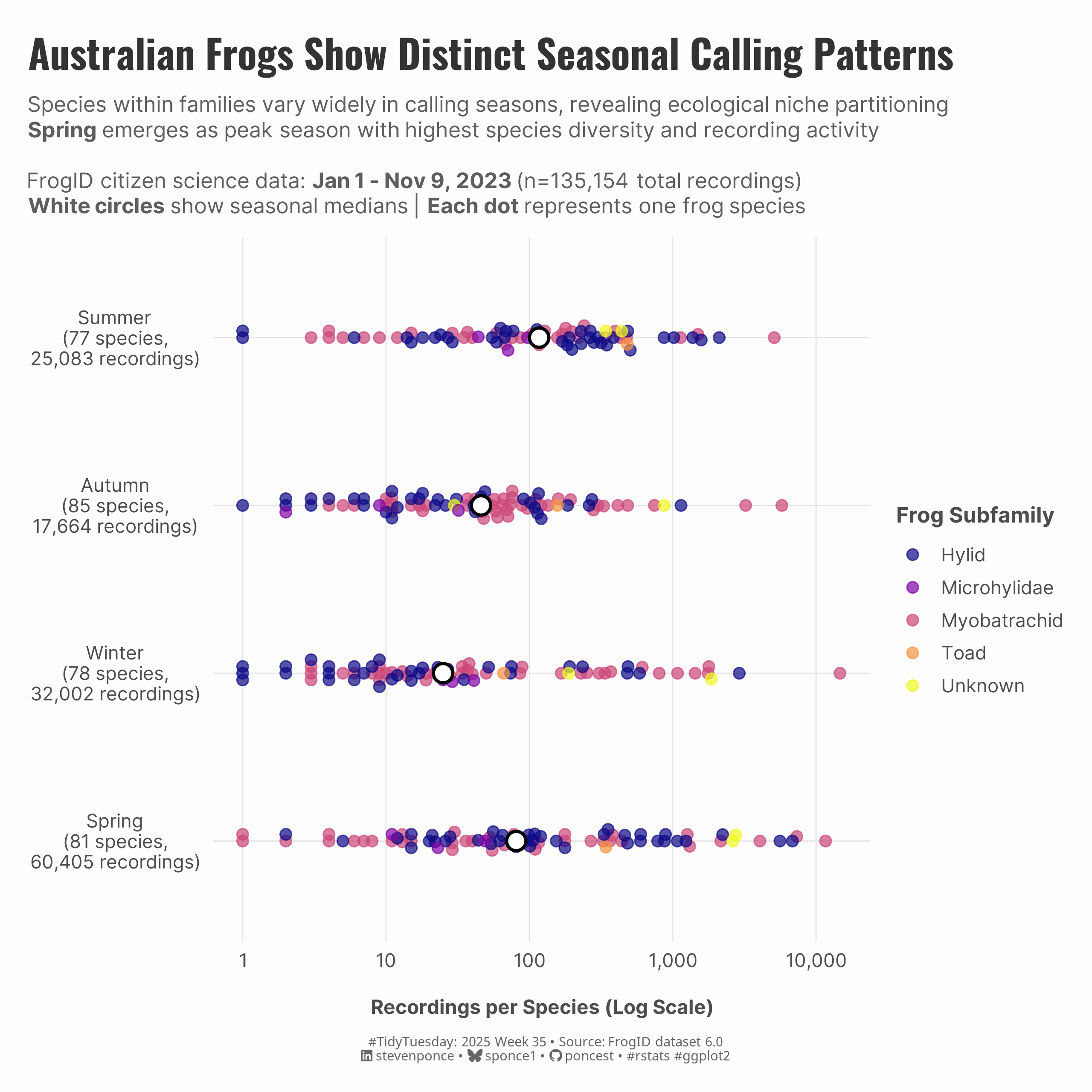{#fig-1}
### <mark> **Steps to Create this Graphic** </mark>
#### 1. Load Packages & Setup
```{r}
#| label: load
#| warning: false
#| message: false
#| results: "hide"

## 1. LOAD PACKAGES & SETUP ----
suppressPackageStartupMessages({
if (!require("pacman")) install.packages("pacman")
pacman::p_load(
    tidyverse,   # Easily Install and Load the 'Tidyverse'
    ggtext,      # Improved Text Rendering Support for 'ggplot2'
    showtext,    # Using Fonts More Easily in R Graphs
    janitor,     # Simple Tools for Examining and Cleaning Dirty Data
    scales,      # Scale Functions for Visualization
    glue,        # Interpreted String Literals,
    ggbeeswarm,  # Categorical Scatter (Violin Point) Plots
    viridis,     # Colorblind-Friendly Color Maps for R
    lubridate    # Make Dealing with Dates a Little Easier
  )})

### |- figure size ----
camcorder::gg_record(
  dir    = here::here("temp_plots"),
  device = "png",
  width  = 8,
  height = 8,
  units  = "in",
  dpi    = 300
)

# Source utility functions
suppressMessages(source(here::here("R/utils/fonts.R")))
source(here::here("R/utils/social_icons.R"))
source(here::here("R/utils/image_utils.R"))
source(here::here("R/themes/base_theme.R"))
```
#### 2. Read in the Data
```{r}
#| label: read
#| include: true
#| eval: true
#| warning: false

tt <- tidytuesdayR::tt_load(2025, week = 35)

frogID_data <- tt$frogID_data |> clean_names()
frog_names <- tt$frog_names |> clean_names()

tidytuesdayR::readme(tt)
rm(tt)
```
#### 3. Examine the Data
```{r}
#| label: examine
#| include: true
#| eval: true
#| results: 'hide'
#| warning: false

glimpse(frogID_data)
glimpse(frog_names)
```
#### 4. Tidy Data
```{r}
#| label: tidy
#| warning: false

frog_data_clean <- frogID_data |>
  rename_all(~ str_replace_all(., "([A-Z])", "_\\1") |> str_to_lower()) |>
  rename_all(~ str_remove(., "^_")) |>
  mutate(
    month = month(event_date, label = TRUE),
    # Define seasons for Southern Hemisphere (Australia)
    season = case_when(
      month %in% c("Dec", "Jan", "Feb") ~ "Summer",
      month %in% c("Mar", "Apr", "May") ~ "Autumn",
      month %in% c("Jun", "Jul", "Aug") ~ "Winter",
      month %in% c("Sep", "Oct", "Nov") ~ "Spring"
    ),
    hour = hour(event_time)
  ) |>
  left_join(frog_names, by = "scientific_name") |>
  mutate(
    common_name = if_else(is.na(common_name) | common_name == "—",
      scientific_name, common_name
    ),
    state_province = str_trim(state_province),
    subfamily_clean = str_trim(coalesce(subfamily, "Unknown"))
  ) |>
  filter(!is.na(state_province), !is.na(season))

# Species seasonal activity
species_seasonal <- frog_data_clean |>
  filter(!is.na(subfamily_clean)) |>
  # Get species with enough records
  group_by(scientific_name) |>
  filter(n() >= 50) |>
  ungroup() |>
  # Count by species and season
  count(scientific_name, common_name, subfamily_clean, season) |>
  # Get top subfamilies
  group_by(subfamily_clean) |>
  mutate(total_subfamily_records = sum(n)) |>
  ungroup() |>
  arrange(desc(total_subfamily_records)) |>
  filter(subfamily_clean %in% unique(subfamily_clean)[1:5]) |> # Top 5 for clarity
  mutate(
    season_ordered = factor(season, levels = c("Spring", "Winter", "Autumn", "Summer"))
  )

# Calculate medians for reference
season_medians <- species_seasonal |>
  group_by(season_ordered) |>
  summarise(median_recordings = median(n), .groups = "drop")

# Add context metrics
season_stats <- species_seasonal |>
  group_by(season_ordered) |>
  summarise(
    total_species = n(),
    total_recordings = sum(n),
    median_recordings = median(n),
    .groups = "drop"
  ) |>
  mutate(
    season_label = paste0(
      season_ordered, "\n(", total_species, " species,\n",
      scales::comma(total_recordings), " recordings)"
    )
  )
```
#### 5. Visualization Parameters
```{r}
#| label: params
#| include: true
#| warning: false

### |-  plot aesthetics ----
# Get basic theme colors
colors <- get_theme_colors()

### |- titles and caption ----
title_text <- str_glue("Australian Frogs Show Distinct Seasonal Calling Patterns")

subtitle_text <- str_glue(
    "Species within families vary widely in calling seasons, revealing ecological niche partitioning<br>",
    "**Spring** emerges as peak season with highest species diversity and recording activity<br><br>",
    "FrogID citizen science data: **Jan 1 - Nov 9, 2023** (n=135,154 total recordings)<br>",
    "**White circles** show seasonal medians | **Each dot** represents one frog species"
)

caption_text <- create_social_caption(
  tt_year = 2025,
  tt_week = 35,
  source_text = "FrogID dataset 6.0"
)

### |-  fonts ----
setup_fonts()
fonts <- get_font_families()

### |-  plot theme ----
# Start with base theme
base_theme <- create_base_theme(colors)

# Add weekly-specific theme elements
weekly_theme <- extend_weekly_theme(
  base_theme,
  theme(
    # Text styling
    plot.title = element_text(face = "bold", family = fonts$title, size = rel(1.2), color = colors$title, margin = margin(b = 10)),
    plot.subtitle = element_text(family = fonts$subtitle, lineheight = 1.2, color = colors$subtitle, size = rel(0.78), margin = margin(b = 20)),

    # Axis elements
    axis.line = element_blank(),
    axis.ticks = element_blank(),

    # Grid elements
    panel.grid.major = element_line(color = "gray90", linetype = "solid", linewidth = 0.3),
    # panel.grid.major.y = element_blank(),
    panel.grid.minor.x = element_blank(),
    panel.grid.minor.y = element_blank(),

    # Axis elements
    axis.text = element_text(color = colors$text, size = rel(0.7)),
    axis.title.x = element_text(color = colors$text, face = "bold", size = rel(0.8), margin = margin(t = 15)),
    axis.title.y = element_text(color = colors$text, face = "bold", size = rel(0.8), margin = margin(r = 10)),

    # Legend elements
    legend.position = "plot",
    legend.title = element_text(family = fonts$tsubtitle, color = colors$text, size = rel(0.8), face = "bold"),
    legend.text = element_text(family = fonts$tsubtitle, color = colors$text, size = rel(0.7)),
    legend.margin = margin(t = 15),

    # Plot margin
    plot.margin = margin(t = 15, r = 15, b = 15, l = 15),
  )
)

# Set theme
theme_set(weekly_theme)
```
#### 6. Plot
```{r}
#| label: plot
#| warning: false

### |-  final plot ----
p <- species_seasonal |>
  ggplot(aes(y = season_ordered, x = n)) +
  # Geoms
  geom_beeswarm(aes(color = subfamily_clean),
    size = 2.5, alpha = 0.7, cex = 1
  ) +
  geom_point(
    data = season_stats,
    aes(y = season_ordered, x = median_recordings),
    shape = 21, size = 4, fill = "white", color = "black", stroke = 1.2
  ) +
  # Scales
  scale_color_viridis_d(name = "Frog Subfamily", option = "plasma") +
  scale_x_log10(labels = comma_format()) +
  scale_y_discrete(labels = season_stats$season_label) +
  # Labs
  labs(
    title = title_text,
    subtitle = subtitle_text,
    caption = caption_text,
    y = NULL,
    x = "Recordings per Species (Log Scale)"
  ) +
  # Theme
  theme(
    axis.text.y = element_text(size = 10, hjust = 0.5),
    legend.position = "right",
    plot.title = element_text(
      size = rel(1.5),
      family = fonts$title,
      face = "bold",
      color = colors$title,
      lineheight = 1.1,
      margin = margin(t = 5, b = 5)
    ),
    plot.subtitle = element_markdown(
      size = rel(0.80),
      family = fonts$subtitle,
      color = alpha(colors$subtitle, 0.9),
      lineheight = 1.2,
      margin = margin(t = 5, b = 10)
    ),
    plot.caption = element_markdown(
      size = rel(0.5),
      family = fonts$caption,
      color = colors$caption,
      hjust = 0.5,
      margin = margin(t = 10)
    )
  )
```
#### 7. Save
```{r}
#| label: save
#| warning: false

### |-  plot image ----
save_plot(
  plot = p,
  type = "tidytuesday",
  year = 2025,
  week = 35,
  width  = 8,
  height = 8
  )
```
#### 8. Session Info
::: {.callout-tip collapse="true"}
##### Expand for Session Info
```{r, echo = FALSE}
#| eval: true
#| warning: false
sessionInfo()
```
:::
#### 9. GitHub Repository
::: {.callout-tip collapse="true"}
##### Expand for GitHub Repo
The complete code for this analysis is available in [`tt_2025_35.qmd`](https://github.com/poncest/personal-website/blob/master/data_visualizations/TidyTuesday/2025/tt_2025_35.qmd).
For the full repository, [click here](https://github.com/poncest/personal-website/).
:::
#### 10. References
::: {.callout-tip collapse="true"}
##### Expand for References
1. Data Sources:
- TidyTuesday 2025 Week 35: \[Australian Frogs\](https://github.com/rfordatascience/tidytuesday/blob/main/data/2025/2025-09-02)
:::
