Galaxy Centers Shift From Mostly Non-Star-Forming to Mostly Star-Forming

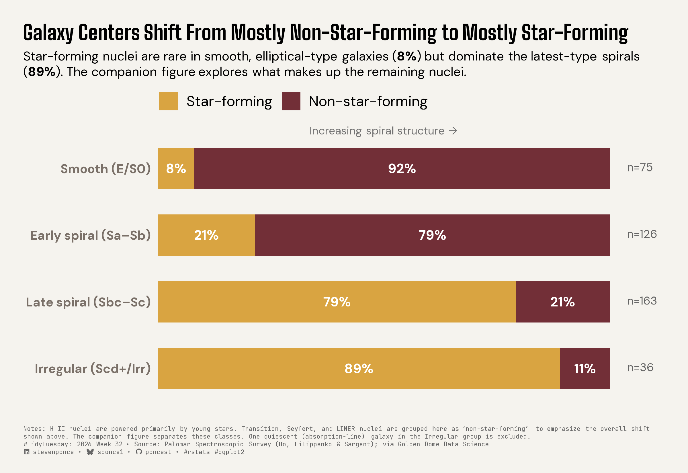
Star-forming nuclei are rare in smooth, elliptical-type galaxies (8%) but dominate the latest-type spirals (89%). The companion figure explores what makes up the remaining nuclei.

This chart shows how the dominant power source of a galaxy’s nucleus shifts across the Hubble sequence, from 8% star-forming in smooth elliptical galaxies to 89% in irregular spirals. Morphology groups are compared using a 100% stacked composition chart with direct sample-size labels. Built in R with ggplot2, ggtext, and ggview.

Figure 1: Horizontal 100% stacked bar chart titled “Galaxy Centers Shift From Mostly Non-Star-Forming to Mostly Star-Forming.” Four galaxy morphology groups, ordered from smooth elliptical galaxies to irregular spirals, show the share of star-forming versus non-star-forming galactic nuclei. Star-forming nuclei are rare in smooth, elliptical-type galaxies at 8 percent (n=75), rise to 21 percent in early spirals (n=126), reach 79 percent in late spirals (n=163), and dominate at 89 percent in irregular galaxies (n=36). Non-star-forming nuclei — which include Seyfert, LINER, and Transition classes — show the mirror pattern, falling from 92 percent to 11 percent across the same sequence. Data from the Palomar Spectroscopic Survey (Ho, Filippenko, and Sargent), via Golden Dome Data Science.

Steps to Create this Graphic

1. Load Packages & Setup

```{r}
#| label: load
#| warning: false
#| message: false      
#| results: "hide"     

## 1. LOAD PACKAGES & SETUP ----
suppressPackageStartupMessages({
if (!require("pacman")) install.packages("pacman")
pacman::p_load(
    tidyverse, ggtext, showtext, janitor, ggrepel,      
    scales, glue, skimr, ggview
    )
})

# Source utility functions
suppressMessages(source(here::here("R/utils/fonts.R")))
source(here::here("R/utils/social_icons.R"))
source(here::here("R/utils/image_utils.R"))
source(here::here("R/themes/base_theme.R"))
```

2. Read in the Data

```{r}
#| label: read
#| include: true
#| eval: true
#| warning: false

## 2. READ IN THE DATA ----
tt <- tidytuesdayR::tt_load(2026, week = 32)
palomar_survey <- tt$palomar_survey
rm(tt)
```

3. Examine the Data

```{r}
#| label: examine
#| include: true
#| eval: true
#| results: 'hide'
#| warning: false

glimpse(palomar_survey)
skim_without_charts(palomar_survey)
```

4. Tidy Data

```{r}
#| label: tidy
#| warning: false

### |- derive broad morphology stage from hubble_type ----
bucket_hubble <- function(h) {
  case_when(
    is.na(h) ~ NA_character_,
    str_detect(h, "^E\\d") | h == "E" ~ "E",
    str_detect(h, "^E\\d?/S0") ~ "S0",
    str_detect(h, "0/a") ~ "Sa",
    str_detect(h, "^(\\(R\\))?(RSB|RSA|SAB|SB|SA|S)?\\(?[a-z]{0,2}\\)?0") ~ "S0",
    str_detect(h, "^I[Bm0]?(\\s|$|\\d)") |
      str_detect(h, "^Im") | str_detect(h, "^IB") | str_detect(h, "^IAB") ~ "Irr",
    TRUE ~ {
      core <- h |>
        str_remove_all("\\((s|r|rs|sr|b|B)\\)") |>
        str_remove("^\\(R\\)") |>
        str_remove("^R") |>
        str_remove("^(SAB|SB|SA|S)") |>
        str_trim()
      stage <- str_extract(str_to_lower(core), "^(cd|bc|ab|dm|a|b|c|d|m)")
      case_when(
        stage == "a" ~ "Sa",  stage == "ab" ~ "Sab", stage == "b" ~ "Sb",
        stage == "bc" ~ "Sbc", stage == "c" ~ "Sc",  stage == "cd" ~ "Scd",
        stage == "d" ~ "Sd",  stage == "dm" ~ "Sdm", stage == "m" ~ "Sm",
        str_detect(str_to_lower(h), "pec") ~ "Pec/Other",
        TRUE ~ "Unclassified"
      )
    }
  )
}

broad_group <- function(stage) {
  case_when(
    stage %in% c("E", "S0") ~ "E/S0",
    stage %in% c("Sa", "Sab", "Sb") ~ "Sa-Sb",
    stage %in% c("Sbc", "Sc") ~ "Sbc-Sc",
    stage %in% c("Scd", "Sd", "Sdm", "Sm", "Irr") ~ "Scd+/Irr",
    TRUE ~ NA_character_
  )
}

survey_tidy <- palomar_survey |>
  clean_names() |>
  mutate(
    stage       = bucket_hubble(hubble_type),
    morph_group = broad_group(stage)
  )

### |- two-process composition by morphology, plain-language labels ----
comp_data <- survey_tidy |>
  filter(
    !is.na(morph_group), !is.na(activity_type),
    activity_type != "Absorption"
  ) |>
  mutate(
    morph_group = factor(morph_group,
      levels = c("E/S0", "Sa-Sb", "Sbc-Sc", "Scd+/Irr"),
      labels = c(
        "Smooth (E/S0)",
        "Early spiral (Sa\u2013Sb)",
        "Late spiral (Sbc\u2013Sc)",
        "Irregular (Scd+/Irr)"
      )
    ),
    bucket = if_else(activity_type == "H II", "Star-forming", "Non-star-forming"),
    bucket = factor(bucket, levels = c("Star-forming", "Non-star-forming"))
  )

comp_summary <- comp_data |>
  summarise(n_total = n(), .by = morph_group) |>
  arrange(morph_group)

comp_pct <- comp_data |>
  summarise(n = n(), .by = c(morph_group, bucket)) |>
  complete(morph_group, bucket, fill = list(n = 0)) |>
  mutate(pct = n / sum(n) * 100, .by = morph_group) |>
  left_join(comp_summary, by = "morph_group")
```

5. Visualization Parameters

```{r}
#| label: params
#| include: true
#| warning: false

## |-  plot aesthetics ----
clrs <- get_theme_colors(
    palette = c(
        "Star-forming"     = "#D9A441",  
        "Non-star-forming" = "#722F37"   
    )
)

### |-  titles and caption ----
title_text <- str_glue("Galaxy Centers Shift From Mostly Non-Star-Forming to Mostly Star-Forming")

subtitle_text <- str_glue(
    "Star-forming nuclei are rare in smooth, elliptical-type galaxies ",
    "(**8%**) but dominate the latest-type spirals (**89%**). The ",
    "companion figure explores what makes up the remaining nuclei."
)

caption_text <- str_glue(
    "Notes: H II nuclei are powered primarily by young stars. Transition, ",
    "Seyfert, and LINER nuclei are grouped here as 'non-star-forming' to ",
    "emphasize the overall shift shown above. The companion figure ",
    "separates these classes. One quiescent (absorption-line) galaxy in ",
    "the Irregular group is excluded.<br>",
    "{create_social_caption(tt_year = 2026, tt_week = 32, source_text = 'Palomar Spectroscopic Survey (Ho, Filippenko & Sargent); via Golden Dome Data Science')}"
)

### |-  fonts ----
setup_fonts()
fonts <- get_font_families()

### |-  plot theme ----
### |- plot theme ----
base_theme <- create_base_theme(clrs)

weekly_theme <- extend_weekly_theme(
  base_theme,
  theme(
    plot.title = element_textbox_simple(
      face = "bold", family = fonts$title_1,
      size = 16, lineheight = 1.2,
      margin = margin(b = 6)
    ),
    plot.subtitle = element_textbox_simple(
      family = fonts$subtitle, size = 10,
      lineheight = 1.3,
      margin = margin(b = 10)
    ),
    plot.caption = element_textbox_simple(
      family = fonts$caption, size = 5,
      color = "gray40", lineheight = 1.3,
      margin = margin(t = 12)
    ),
    plot.margin = margin(t = 20, r = 20, b = 15, l = 20),
    axis.text.y = element_text(face = "bold", size = 10),
    axis.text.x = element_blank(),
    axis.title = element_blank(),
    axis.ticks = element_blank(),
    panel.grid = element_blank(),
    legend.position = "top",
    legend.justification = "left",
    legend.title = element_blank(),
    legend.margin = margin(t = 0, b = 4),
    legend.box.spacing = unit(2, "pt")
  )
)

theme_set(weekly_theme)
```

6. Plot

```{r}
#| label: plot
#| warning: false

### |- plot----
comp_pct <- comp_pct |>
  mutate(label = if_else(pct >= 6, str_glue("{round(pct)}%"), ""))

p <- ggplot(comp_pct, aes(x = pct, y = fct_rev(morph_group), fill = bucket)) +
  geom_col(width = 0.62, position = position_stack(reverse = TRUE)) +
  geom_text(
    aes(label = label),
    position = position_stack(vjust = 0.5, reverse = TRUE),
    color = "white", size = 3.6, family = fonts$text, fontface = "bold"
  ) +
  geom_richtext(
    data = comp_summary,
    aes(x = 103, y = fct_rev(morph_group), label = str_glue("n={n_total}")),
    inherit.aes = FALSE, fill = NA, label.color = NA, hjust = 0,
    size = 3.2, family = fonts$text, color = "gray40"
  ) +
  annotate(
    "richtext",
    x = 50, y = 4.55, label = "Increasing spiral structure \u2192",
    fill = NA, label.color = NA, hjust = 0.5, size = 3.1, color = "gray45",
    family = fonts$text
  ) +
  scale_fill_manual(values = c("Star-forming" = "#D9A441", "Non-star-forming" = "#722F37")) +
  scale_x_continuous(limits = c(0, 112), expand = expansion(mult = 0)) +
  scale_y_discrete(expand = expansion(add = c(0.65, 0.75))) +
  labs(title = title_text, subtitle = subtitle_text, caption = caption_text) +
  guides(fill = guide_legend(nrow = 1)) +
  canvas(width = 8, height = 5.5, units = "in", dpi = 300)
```

7. Save

```{r}
#| label: save
#| warning: false

### |- save ----
main_path  <- here::here("data_visualizations", "TidyTuesday", "2026", "tt_2026_32.png")
thumb_path <- here::here("data_visualizations", "TidyTuesday", "2026", "thumbnails", "tt_2026_32.png")

# Full-size version, for the QMD figure
save_ggplot(
  plot = p,
  file = main_path,
  width = 8,
  height = 5.5,
  units = "in",
  dpi = 300,
  create.dir = TRUE
)

# Reduced-size thumbnail, for the YAML `image:` field
fs::dir_create(dirname(thumb_path))
magick::image_read(main_path) |>
  magick::image_resize("400") |>
  magick::image_write(thumb_path)
```

8. Session Info

TipExpand for Session Info

R version 4.6.1 (2026-06-24)
Platform: aarch64-apple-darwin23
Running under: macOS Tahoe 26.5.2

Matrix products: default
BLAS:   /Library/Frameworks/R.framework/Versions/4.6/Resources/lib/libRblas.0.dylib 
LAPACK: /Library/Frameworks/R.framework/Versions/4.6/Resources/lib/libRlapack.dylib;  LAPACK version 3.12.1

locale:
[1] en_US.UTF-8/en_US.UTF-8/en_US.UTF-8/C/en_US.UTF-8/en_US.UTF-8

time zone: America/New_York
tzcode source: internal

attached base packages:
[1] stats     graphics  grDevices utils     datasets  methods   base     

other attached packages:
 [1] here_1.0.2      ggview_0.2.2    skimr_2.2.2     glue_1.8.1     
 [5] scales_1.4.0    ggrepel_0.9.8   janitor_2.2.1   showtext_0.9-8 
 [9] showtextdb_3.0  sysfonts_0.8.9  ggtext_0.1.2    lubridate_1.9.5
[13] forcats_1.0.1   stringr_1.6.0   dplyr_1.2.1     purrr_1.2.2    
[17] readr_2.2.0     tidyr_1.3.2     tibble_3.3.1    ggplot2_4.0.3  
[21] tidyverse_2.0.0 pacman_0.5.1   

loaded via a namespace (and not attached):
 [1] gtable_0.3.6       xfun_0.60          httr2_1.3.0        htmlwidgets_1.6.4 
 [5] gh_1.6.1           tzdb_0.5.0         vctrs_0.7.3        tools_4.6.1       
 [9] generics_0.1.4     parallel_4.6.1     curl_7.1.0         pkgconfig_2.0.3   
[13] RColorBrewer_1.1-3 S7_0.2.2           lifecycle_1.0.5    compiler_4.6.1    
[17] farver_2.1.2       textshaping_1.0.5  repr_1.1.7         codetools_0.2-20  
[21] snakecase_0.11.1   litedown_0.10      htmltools_0.5.9    yaml_2.3.12       
[25] crayon_1.5.3       pillar_1.11.1      magick_2.9.1       commonmark_2.0.0  
[29] tidyselect_1.2.1   digest_0.6.39      stringi_1.8.7      labeling_0.4.3    
[33] rprojroot_2.1.1    fastmap_1.2.0      grid_4.6.1         cli_3.6.6         
[37] magrittr_2.0.5     base64enc_0.1-6    withr_3.0.3        bit64_4.8.2       
[41] timechange_0.4.0   rmarkdown_2.31     tidytuesdayR_1.3.2 gitcreds_0.1.2    
[45] bit_4.6.0          otel_0.2.0         ragg_1.5.2         hms_1.1.4         
[49] evaluate_1.0.5     knitr_1.51         markdown_2.0       rlang_1.3.0       
[53] gridtext_0.1.6     Rcpp_1.1.2         xml2_1.6.0         rstudioapi_0.19.0 
[57] vroom_1.7.1        jsonlite_2.0.0     R6_2.6.1           fs_2.1.0          
[61] systemfonts_1.3.2 

9. GitHub Repository

TipExpand for GitHub Repo

The complete code for this analysis is available in tt_2026_32.qmd.

For the full repository, click here.

10. References

TipExpand for References

1. Data Source:
   • TidyTuesday 2026 Week 32: the Palomar Spectroscopic Survey of Nearby Galaxies

11. Custom Functions Documentation

Note📦 Custom Helper Functions

This analysis uses custom functions from my personal module library for efficiency and consistency across projects.

Functions Used:

• fonts.R: setup_fonts(), get_font_families() - Font management with showtext
• social_icons.R: create_social_caption() - Generates formatted social media captions
• image_utils.R: save_plot() - Consistent plot saving with naming conventions
• base_theme.R: create_base_theme(), extend_weekly_theme(), get_theme_colors() - Custom ggplot2 themes

Why custom functions?
These utilities standardize theming, fonts, and output across all my data visualizations. The core analysis (data tidying and visualization logic) uses only standard tidyverse packages.

Source Code:
View all custom functions → GitHub: R/utils