Steven Ponce home pageSteven Ponce home page Steven Ponce
  • About
  • Data Visualizations
  • Projects
  • Behind the Viz
  • Resume
  • Email

On this page

  • Steps to Create this Graphic
    • 1. Load Packages & Setup
    • 2. Read in the Data
    • 3. Examine the Data
    • 4. Tidy Data
    • 5. Visualization Parameters
    • 6. Plot
    • 7. Save
    • 8. Session Info
    • 9. GitHub Repository

The Rise and Fall of Bob’s Burgers Ratings Across Seasons

  • Show All Code
  • Hide All Code

  • View Source

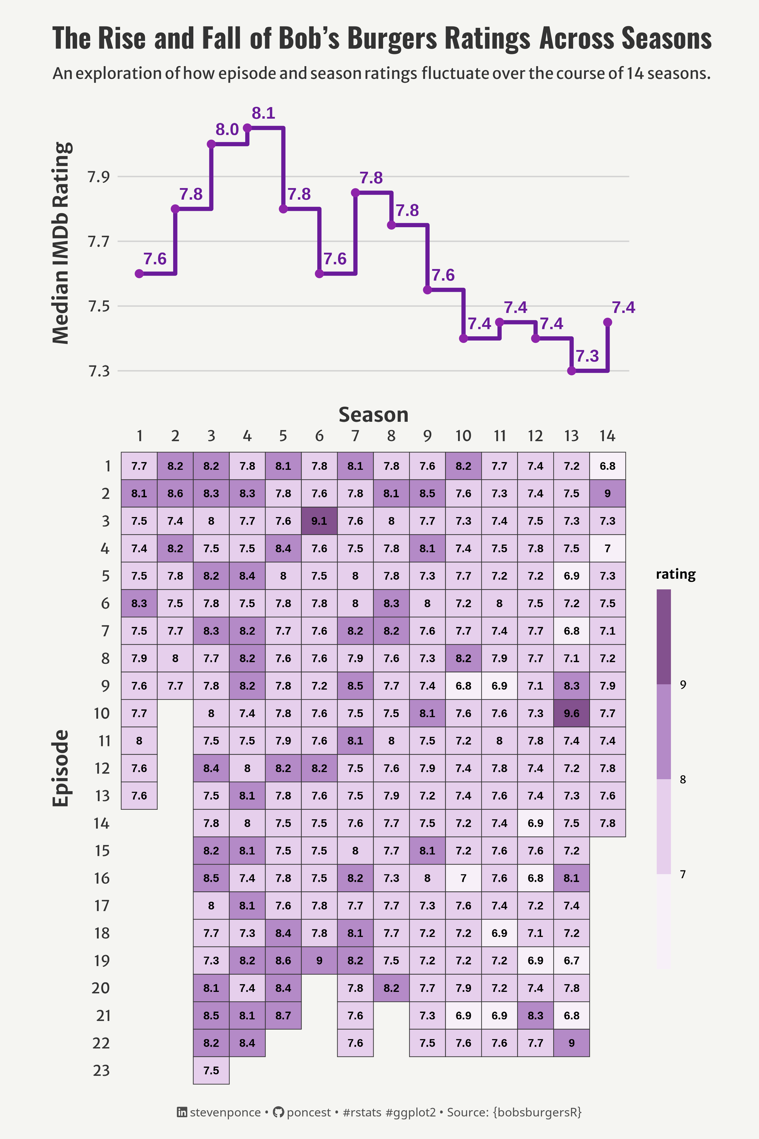
An exploration of how episode and season ratings fluctuate over the course of 14 seasons.

Standalone Visualization
Bob's Burgers
2024
Bob’s Burgers episode and season ratings across 14 seasons. Built in R.
Author

Steven Ponce

Published

October 27, 2024

Figure 1: Line chart and heatmap showing IMDb ratings for Bob’s Burgers across seasons and episodes.

Steps to Create this Graphic

1. Load Packages & Setup

Show code
```{r}
#| label: load
#| warning: false

## 1. LOAD PACKAGES & SETUP ----
if (!require("pacman")) install.packages("pacman")
pacman::p_load(
  tidyverse,         # Easily Install and Load the 'Tidyverse'
  ggtext,            # Improved Text Rendering Support for 'ggplot2'
  showtext,          # Using Fonts More Easily in R Graphs
  janitor,           # Simple Tools for Examining and Cleaning Dirty Data
  skimr,             # Compact and Flexible Summaries of Data
  scales,            # Scale Functions for Visualization
  glue,              # Interpreted String Literals
  colorspace,        # A Toolbox for Manipulating and Assessing Colors and Palettes
  patchwork,         # The Composer of Plots
  bobsburgersR       # Bob's Burgers Datasets for Data Visualization
)  

### |- resolution ----
showtext_opts(dpi = 320, regular.wt = 300, bold.wt = 800)
```

2. Read in the Data

Show code
```{r}
#| label: read
#| include: true
#| eval: true
#| results: 'hide'
#| warning: false

bobsburgersR::imdb_wikipedia_data
```

3. Examine the Data

Show code
```{r}
#| label: examine
#| include: true
#| eval: true
#| results: 'hide'
#| warning: false

glimpse(imdb_wikipedia_data)
skim(imdb_wikipedia_data)
```

4. Tidy Data

Show code
```{r}
#| label: tidy
#| warning: false

### |- heatmap data ----
heatmap_data <- imdb_wikipedia_data |>
  mutate(
    season = factor(season),
    episode = factor(episode, levels = rev(unique(episode))),
  ) |>
  filter(!is.na(rating))

### |- heatmap data ----
linechart_data <- imdb_wikipedia_data |>
  group_by(season) |>
  summarize(
    median_rating = median(rating, na.rm = TRUE),
    .groups = "drop"
  ) |>
  mutate(season = factor(season))
```

5. Visualization Parameters

Show code
```{r}
#| label: params
#| include: true
#| warning: false

### |- plot aesthetics ----
bkg_col      <- "#f5f5f2"    
title_col    <- "gray20"           
subtitle_col <- "gray20"     
caption_col  <- "gray30"   
text_col     <- "gray20"    
col_palette  <- c("#F9F6FB", "#F0DDF1", "#D6B9E3", "#B78FCA", "#9D5CAA", "#684671")

### |-  titles and caption ----

# icons
tt <- str_glue("Source: {{bobsburgersR}}")
li <- str_glue("<span style='font-family:fa6-brands'>&#xf08c;</span>")
gh <- str_glue("<span style='font-family:fa6-brands'>&#xf09b;</span>")

# text
title_text    <- str_glue("The Rise and Fall of Bob's Burgers Ratings Across Seasons")
subtitle_text <- str_glue("An exploration of how episode and season ratings fluctuate over the course of 14 seasons.")
caption_text  <- str_glue("{li} stevenponce &bull; {gh} poncest &bull; #rstats #ggplot2 &bull; {tt}")

### |-  fonts ----
font_add("fa6-brands", here::here("fonts/6.4.2/Font Awesome 6 Brands-Regular-400.otf"))
font_add_google("Oswald", regular.wt = 400, family = "title")
font_add_google("Merriweather Sans", regular.wt = 400, family = "subtitle")
font_add_google("Merriweather Sans", regular.wt = 400, family = "text")
font_add_google("Noto Sans", regular.wt = 400, family = "caption")
showtext_auto(enable = TRUE)

### |-  plot theme ----
theme_set(theme_minimal(base_size = 14, base_family = "text"))                

theme_update(
  plot.title.position   = "plot",
  plot.caption.position = "plot",
  legend.position       = 'plot',
  plot.background       = element_rect(fill = bkg_col, color = bkg_col),
  panel.background      = element_rect(fill = bkg_col, color = bkg_col),
  plot.margin           = margin(t = 10, r = 20, b = 10, l = 20),
  axis.title.x          = element_text(margin = margin(10, 0, 0, 0), size = rel(1.1), 
                                       color = text_col, family = "text", face = "bold", hjust = 0.5),
  axis.title.y          = element_text(margin = margin(0, 10, 0, 0), size = rel(1.1), 
                                       color = text_col, family = "text", face = "bold", hjust = 0.5),
  axis.text             = element_text(size = rel(0.8), color = text_col, family = "text"),
  panel.grid.major.y    = element_line(color = "#d3d3d3", linewidth = 0.5), 
  panel.grid.major.x    = element_blank(), 
  panel.grid.minor      = element_blank()
)  
```

6. Plot

Show code
```{r}
#| label: plot
#| warning: false

### |-  line chart ----
line_chart <- linechart_data |>
  ggplot(aes(x = season, y = median_rating, group = 1)) +

  # Geoms
  geom_step(color = "#6a1b9a", linewidth = 1.5) +
  geom_point(color = "#8e24aa", size = 4, shape = 20) +
  geom_text(aes(label = format(round(median_rating, 1), nsmall = 1)),
    hjust = -0.2, vjust = -0.8, size = 4.5, color = "#6a1b9a", fontface = "bold"
  ) +

  # Scales
  scale_x_discrete() +
  scale_y_continuous(
    labels = scales::label_number(accuracy = 0.1),
    expand = expansion(mult = c(0, 0.05))
  ) +
  coord_cartesian(clip = "off") +

  # Labs
  labs(
    x = NULL,
    y = "Median IMDb Rating",
  ) +

  # Theme
  theme(
    axis.text.x = element_blank()
  )


### |-  heatmap plot ----
heatmap_plot <- heatmap_data |>
  ggplot(aes(x = season, y = episode, fill = rating)) +

  # Geoms
  geom_tile(linewidth = 0.25, color = "grey20") +
  geom_text(aes(label = round(rating, 1)),
    color = "black",
    size = 3,
    fontface = "bold"
  ) +

  # Scales
  scale_x_discrete(position = "top") +
  scale_y_discrete() +
  scale_fill_stepsn(
    colors = col_palette,
    breaks = c(1, 2, 3, 4, 5, 6, 7, 8, 9, 10),
    transform = "identity",
    guide = guide_colorsteps(
      barheight = unit(20, "lines"),
      barwidth = unit(.75, "lines")
    )
  ) +
  coord_cartesian(clip = "off") +

  # Labs
  labs(
    x = "Season",
    y = "Episode",
  ) +

  # Theme
  theme(
    legend.position    = "right",
    legend.title       = element_text(size = 10, face = "bold"),
    legend.text        = element_text(size = 8),
    panel.grid.major.y = element_blank(),
    panel.grid.minor.y = element_blank(),
    panel.grid         = element_blank(),
  )


### |-  combined plots ----  
combined_plot <- (line_chart / heatmap_plot) +
  patchwork::plot_layout(
    heights = c(0.5, 1.25),
  ) +

  # Labs
  plot_annotation(
    title = title_text,
    subtitle = subtitle_text,
    caption = caption_text
  ) &

  # Theme
  theme(
    plot.margin  = margin(10, 20, 10, 20),
    plot.title   = element_markdown(
      size       = rel(1.5),
      family     = "title",
      face       = "bold",
      color      = title_col,
      lineheight = 1.1,
      margin     = margin(t = 10, b = 5)
    ),
    plot.subtitle = element_markdown(
      size       = rel(0.85),
      family     = "subtitle",
      color      = subtitle_col,
      lineheight = 1.1,
      margin     = margin(t = 5, b = 15)
    ),
    plot.caption = element_markdown(
      size       = rel(0.65),
      family     = "caption",
      color      = caption_col,
      lineheight = 1.1,
      hjust      = 0.5,
      halign     = 0.5,
      margin     = margin(t = 5, b = 5)
    )
  )
```

7. Save

Show code
```{r}
#| label: save
#| warning: false

### |-  plot image ----  

# Save the plot as PNG
ggsave(
  filename = here::here("projects/standalone_visualizations/sa_2024-10-27.png"), 
  plot = combined_plot,
  width = 8, height = 12, units = "in", dpi = 320
)

### |-  plot thumbnail----  
magick::image_read(here::here("projects/standalone_visualizations/sa_2024-10-27.png")) |> 
  magick::image_resize(geometry = "400") |> 
  magick::image_write(here::here("projects/standalone_visualizations/thumbnails/sa_2024-10-27.png"))
```

8. Session Info

TipExpand for Session Info
R version 4.4.1 (2024-06-14 ucrt)
Platform: x86_64-w64-mingw32/x64
Running under: Windows 11 x64 (build 22631)

Matrix products: default


locale:
[1] LC_COLLATE=English_United States.utf8 
[2] LC_CTYPE=English_United States.utf8   
[3] LC_MONETARY=English_United States.utf8
[4] LC_NUMERIC=C                          
[5] LC_TIME=English_United States.utf8    

time zone: America/New_York
tzcode source: internal

attached base packages:
[1] stats     graphics  grDevices datasets  utils     methods   base     

other attached packages:
 [1] bobsburgersR_0.0.0.9000 patchwork_1.3.0         colorspace_2.1-1       
 [4] glue_1.8.0              scales_1.3.0            skimr_2.1.5            
 [7] janitor_2.2.0           showtext_0.9-7          showtextdb_3.0         
[10] sysfonts_0.8.9          ggtext_0.1.2            lubridate_1.9.3        
[13] forcats_1.0.0           stringr_1.5.1           dplyr_1.1.4            
[16] purrr_1.0.2             readr_2.1.5             tidyr_1.3.1            
[19] tibble_3.2.1            ggplot2_3.5.1           tidyverse_2.0.0        
[22] pacman_0.5.1           

loaded via a namespace (and not attached):
 [1] gtable_0.3.6      xfun_0.49         htmlwidgets_1.6.4 tzdb_0.5.0       
 [5] vctrs_0.6.5       tools_4.4.0       generics_0.1.3    curl_6.0.0       
 [9] fansi_1.0.6       pkgconfig_2.0.3   lifecycle_1.0.4   compiler_4.4.0   
[13] farver_2.1.2      textshaping_0.4.0 munsell_0.5.1     repr_1.1.7       
[17] codetools_0.2-20  snakecase_0.11.1  htmltools_0.5.8.1 yaml_2.3.10      
[21] pillar_1.9.0      magick_2.8.5      commonmark_1.9.2  tidyselect_1.2.1 
[25] digest_0.6.37     stringi_1.8.4     labeling_0.4.3    rprojroot_2.0.4  
[29] fastmap_1.2.0     grid_4.4.0        here_1.0.1        cli_3.6.4        
[33] magrittr_2.0.3    base64enc_0.1-3   utf8_1.2.4        withr_3.0.2      
[37] timechange_0.3.0  rmarkdown_2.29    ragg_1.3.3        hms_1.1.3        
[41] evaluate_1.0.1    knitr_1.49        markdown_1.13     rlang_1.1.6      
[45] gridtext_0.1.5    Rcpp_1.0.13-1     xml2_1.3.6        renv_1.0.3       
[49] rstudioapi_0.17.1 jsonlite_1.8.9    R6_2.5.1          systemfonts_1.1.0

9. GitHub Repository

TipExpand for GitHub Repo

Access the GitHub repository here

Back to top
Source Code
---
freeze: true
title: "The Rise and Fall of Bob's Burgers Ratings Across Seasons"
subtitle: "An exploration of how episode and season ratings fluctuate over the course of 14 seasons."
author: "Steven Ponce"
description: "Bob's Burgers episode and season ratings across 14 seasons. Built in R."
date: "2024-10-27"
categories: ["Standalone Visualization", "Bob's Burgers", "2024"]
image: "thumbnails/sa_2024-10-27.png"
format:
  html:
    toc: true
    toc-depth: 5
    code-link: true
    code-fold: true
    code-tools: true
    code-summary: "Show code"
editor_options: 
  
  chunk_output_type: inline
execute: 
  
  error: false
  message: false
  warning: false
  eval: true
# share:
#   permalink: "https://stevenponce.netlify.app/projects.html"
#   linkedin: true
#   twitter: true
#   email: true
---

![Line chart and heatmap showing IMDb ratings for Bob's Burgers across seasons and episodes.](sa_2024-10-27){#fig-1}

### <mark> __Steps to Create this Graphic__ </mark>

#### 1. Load Packages & Setup 

```{r}
#| label: load
#| warning: false

## 1. LOAD PACKAGES & SETUP ----
if (!require("pacman")) install.packages("pacman")
pacman::p_load(
  tidyverse,         # Easily Install and Load the 'Tidyverse'
  ggtext,            # Improved Text Rendering Support for 'ggplot2'
  showtext,          # Using Fonts More Easily in R Graphs
  janitor,           # Simple Tools for Examining and Cleaning Dirty Data
  skimr,             # Compact and Flexible Summaries of Data
  scales,            # Scale Functions for Visualization
  glue,              # Interpreted String Literals
  colorspace,        # A Toolbox for Manipulating and Assessing Colors and Palettes
  patchwork,         # The Composer of Plots
  bobsburgersR       # Bob's Burgers Datasets for Data Visualization
)  

### |- resolution ----
showtext_opts(dpi = 320, regular.wt = 300, bold.wt = 800)
```

#### 2. Read in the Data 

```{r}
#| label: read
#| include: true
#| eval: true
#| results: 'hide'
#| warning: false

bobsburgersR::imdb_wikipedia_data
```

#### 3. Examine the Data

```{r}
#| label: examine
#| include: true
#| eval: true
#| results: 'hide'
#| warning: false

glimpse(imdb_wikipedia_data)
skim(imdb_wikipedia_data)
```

#### 4. Tidy Data 

```{r}
#| label: tidy
#| warning: false

### |- heatmap data ----
heatmap_data <- imdb_wikipedia_data |>
  mutate(
    season = factor(season),
    episode = factor(episode, levels = rev(unique(episode))),
  ) |>
  filter(!is.na(rating))

### |- heatmap data ----
linechart_data <- imdb_wikipedia_data |>
  group_by(season) |>
  summarize(
    median_rating = median(rating, na.rm = TRUE),
    .groups = "drop"
  ) |>
  mutate(season = factor(season))
```


#### 5. Visualization Parameters 

```{r}
#| label: params
#| include: true
#| warning: false

### |- plot aesthetics ----
bkg_col      <- "#f5f5f2"    
title_col    <- "gray20"           
subtitle_col <- "gray20"     
caption_col  <- "gray30"   
text_col     <- "gray20"    
col_palette  <- c("#F9F6FB", "#F0DDF1", "#D6B9E3", "#B78FCA", "#9D5CAA", "#684671")

### |-  titles and caption ----

# icons
tt <- str_glue("Source: {{bobsburgersR}}")
li <- str_glue("<span style='font-family:fa6-brands'>&#xf08c;</span>")
gh <- str_glue("<span style='font-family:fa6-brands'>&#xf09b;</span>")

# text
title_text    <- str_glue("The Rise and Fall of Bob's Burgers Ratings Across Seasons")
subtitle_text <- str_glue("An exploration of how episode and season ratings fluctuate over the course of 14 seasons.")
caption_text  <- str_glue("{li} stevenponce &bull; {gh} poncest &bull; #rstats #ggplot2 &bull; {tt}")

### |-  fonts ----
font_add("fa6-brands", here::here("fonts/6.4.2/Font Awesome 6 Brands-Regular-400.otf"))
font_add_google("Oswald", regular.wt = 400, family = "title")
font_add_google("Merriweather Sans", regular.wt = 400, family = "subtitle")
font_add_google("Merriweather Sans", regular.wt = 400, family = "text")
font_add_google("Noto Sans", regular.wt = 400, family = "caption")
showtext_auto(enable = TRUE)

### |-  plot theme ----
theme_set(theme_minimal(base_size = 14, base_family = "text"))                

theme_update(
  plot.title.position   = "plot",
  plot.caption.position = "plot",
  legend.position       = 'plot',
  plot.background       = element_rect(fill = bkg_col, color = bkg_col),
  panel.background      = element_rect(fill = bkg_col, color = bkg_col),
  plot.margin           = margin(t = 10, r = 20, b = 10, l = 20),
  axis.title.x          = element_text(margin = margin(10, 0, 0, 0), size = rel(1.1), 
                                       color = text_col, family = "text", face = "bold", hjust = 0.5),
  axis.title.y          = element_text(margin = margin(0, 10, 0, 0), size = rel(1.1), 
                                       color = text_col, family = "text", face = "bold", hjust = 0.5),
  axis.text             = element_text(size = rel(0.8), color = text_col, family = "text"),
  panel.grid.major.y    = element_line(color = "#d3d3d3", linewidth = 0.5), 
  panel.grid.major.x    = element_blank(), 
  panel.grid.minor      = element_blank()
)  
```


#### 6. Plot 

```{r}
#| label: plot
#| warning: false

### |-  line chart ----
line_chart <- linechart_data |>
  ggplot(aes(x = season, y = median_rating, group = 1)) +

  # Geoms
  geom_step(color = "#6a1b9a", linewidth = 1.5) +
  geom_point(color = "#8e24aa", size = 4, shape = 20) +
  geom_text(aes(label = format(round(median_rating, 1), nsmall = 1)),
    hjust = -0.2, vjust = -0.8, size = 4.5, color = "#6a1b9a", fontface = "bold"
  ) +

  # Scales
  scale_x_discrete() +
  scale_y_continuous(
    labels = scales::label_number(accuracy = 0.1),
    expand = expansion(mult = c(0, 0.05))
  ) +
  coord_cartesian(clip = "off") +

  # Labs
  labs(
    x = NULL,
    y = "Median IMDb Rating",
  ) +

  # Theme
  theme(
    axis.text.x = element_blank()
  )


### |-  heatmap plot ----
heatmap_plot <- heatmap_data |>
  ggplot(aes(x = season, y = episode, fill = rating)) +

  # Geoms
  geom_tile(linewidth = 0.25, color = "grey20") +
  geom_text(aes(label = round(rating, 1)),
    color = "black",
    size = 3,
    fontface = "bold"
  ) +

  # Scales
  scale_x_discrete(position = "top") +
  scale_y_discrete() +
  scale_fill_stepsn(
    colors = col_palette,
    breaks = c(1, 2, 3, 4, 5, 6, 7, 8, 9, 10),
    transform = "identity",
    guide = guide_colorsteps(
      barheight = unit(20, "lines"),
      barwidth = unit(.75, "lines")
    )
  ) +
  coord_cartesian(clip = "off") +

  # Labs
  labs(
    x = "Season",
    y = "Episode",
  ) +

  # Theme
  theme(
    legend.position    = "right",
    legend.title       = element_text(size = 10, face = "bold"),
    legend.text        = element_text(size = 8),
    panel.grid.major.y = element_blank(),
    panel.grid.minor.y = element_blank(),
    panel.grid         = element_blank(),
  )


### |-  combined plots ----  
combined_plot <- (line_chart / heatmap_plot) +
  patchwork::plot_layout(
    heights = c(0.5, 1.25),
  ) +

  # Labs
  plot_annotation(
    title = title_text,
    subtitle = subtitle_text,
    caption = caption_text
  ) &

  # Theme
  theme(
    plot.margin  = margin(10, 20, 10, 20),
    plot.title   = element_markdown(
      size       = rel(1.5),
      family     = "title",
      face       = "bold",
      color      = title_col,
      lineheight = 1.1,
      margin     = margin(t = 10, b = 5)
    ),
    plot.subtitle = element_markdown(
      size       = rel(0.85),
      family     = "subtitle",
      color      = subtitle_col,
      lineheight = 1.1,
      margin     = margin(t = 5, b = 15)
    ),
    plot.caption = element_markdown(
      size       = rel(0.65),
      family     = "caption",
      color      = caption_col,
      lineheight = 1.1,
      hjust      = 0.5,
      halign     = 0.5,
      margin     = margin(t = 5, b = 5)
    )
  )

```


#### 7. Save

```{r}
#| label: save
#| warning: false

### |-  plot image ----  

# Save the plot as PNG
ggsave(
  filename = here::here("projects/standalone_visualizations/sa_2024-10-27.png"), 
  plot = combined_plot,
  width = 8, height = 12, units = "in", dpi = 320
)

### |-  plot thumbnail----  
magick::image_read(here::here("projects/standalone_visualizations/sa_2024-10-27.png")) |> 
  magick::image_resize(geometry = "400") |> 
  magick::image_write(here::here("projects/standalone_visualizations/thumbnails/sa_2024-10-27.png"))
```


#### 8. Session Info

::: {.callout-tip collapse="true"}
##### Expand for Session Info

```{r, echo = FALSE}
#| eval: true
#| warning: false

sessionInfo()
```
:::

#### 9. GitHub Repository

::: {.callout-tip collapse="true"}

##### Expand for GitHub Repo
 
[Access the GitHub repository here](https://github.com/poncest/personal-website/)
:::
© 2024–2026 Steven Ponce · Built with R + Quarto

Source Issues