Bob’s Burgers: The Fart Report

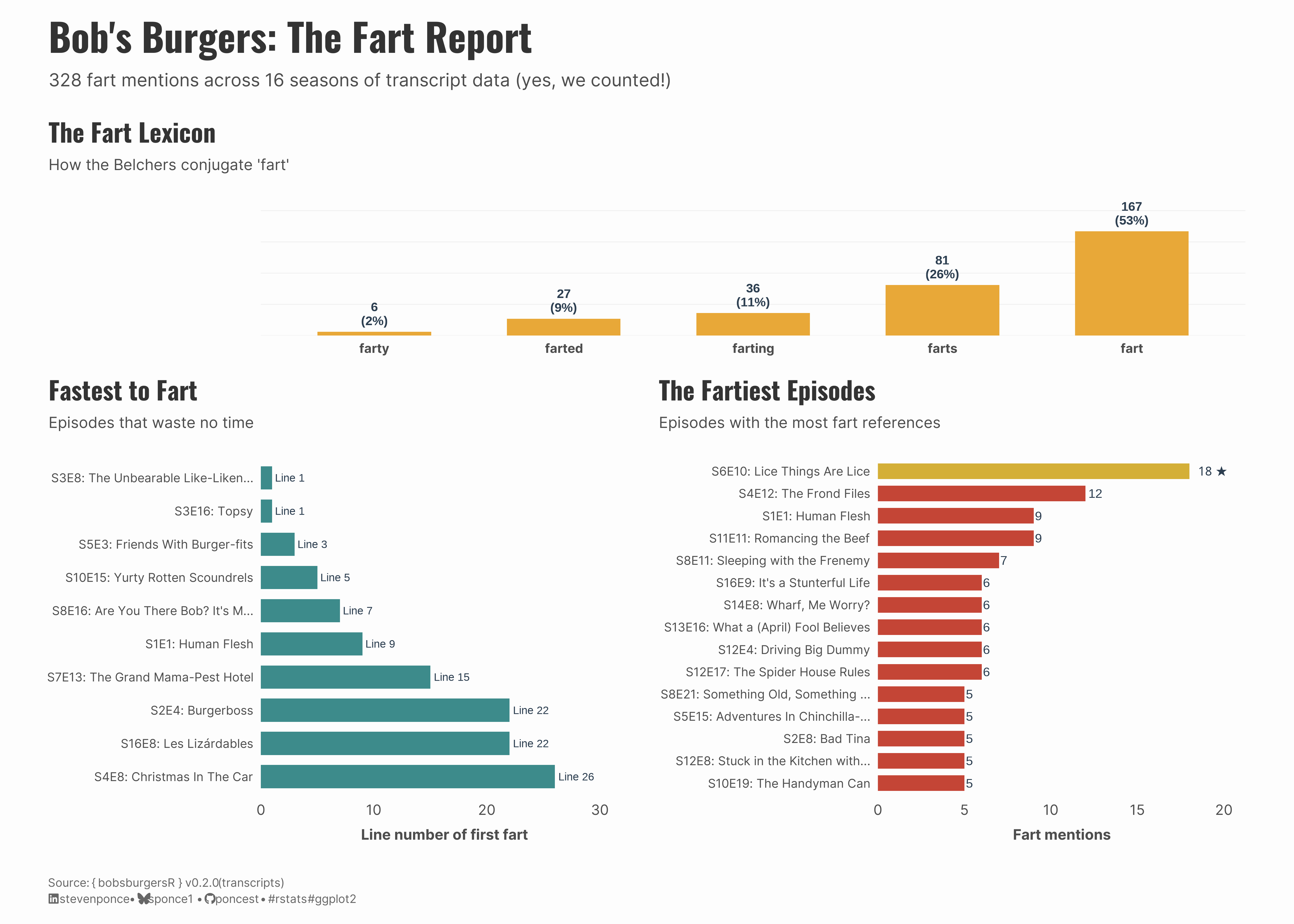
328 fart mentions across 16 seasons of transcript data (yes, we counted!)

A playful analysis of flatulence in Bob’s Burgers using transcript data from the bobsburgersR package. Exploring the fart lexicon, fastest-to-fart episodes, and the show’s fartiest moments.

Figure 1: Three-panel data visualization titled ‘Bob’s Burgers: The Fart Report’ analyzing 328 fart mentions across 16 seasons. The top panel shows ‘The Fart Lexicon’ with vertical bars: ‘fart’ dominates at 53%, followed by ‘farts’ (26%), ‘farting’ (11%), ‘farted’ (9%), and ‘farty’ (2%). Bottom left shows ‘Fastest to Fart’ episodes, with S3E8 and S3E16 achieving the first fart by Line 1. Bottom right shows ‘The Fartiest Episodes’ with S6E10 ‘Lice Things Are Lice’ leading at 18 mentions, highlighted in gold. Color palette uses mustard yellow, teal, and red.

Steps to Create this Graphic

1. Load Packages & Setup

```{r}
#| label: load
#| warning: false
#| message: false
#| results: "hide"

## 1. LOAD PACKAGES & SETUP ----
suppressPackageStartupMessages({
if (!require("pacman")) install.packages("pacman")
pacman::p_load(
  tidyverse,         # Easily Install and Load the 'Tidyverse'
  ggtext,            # Improved Text Rendering Support for 'ggplot2'
  showtext,          # Using Fonts More Easily in R Graphs
  janitor,           # Simple Tools for Examining and Cleaning Dirty Data
  skimr,             # Compact and Flexible Summaries of Data
  scales,            # Scale Functions for Visualization
  glue,              # Interpreted String Literals
  patchwork,         # The Composer of Plots
  bobsburgersR       # Bob's Burgers Datasets for Data Visualization
)  
})

### |- figure size ----
camcorder::gg_record(
  dir    = here::here("temp_plots"),
  device = "png",
  width  = 14,
  height = 10,
  units  = "in",
  dpi    = 320
)

# Source utility functions
suppressMessages(source(here::here("R/utils/fonts.R")))
source(here::here("R/utils/social_icons.R"))
source(here::here("R/utils/image_utils.R"))
source(here::here("R/themes/base_theme.R"))
```

2. Read in the Data

```{r}
#| label: read
#| include: true
#| eval: true
#| warning: false

transcript_data <- bobsburgersR::transcript_data
```

3. Examine the Data

```{r}
#| label: examine
#| include: true
#| eval: true
#| results: 'hide'
#| warning: false

glimpse(transcript_data)
skim_without_charts(transcript_data)
```

4. Tidy Data

```{r}
#| label: tidy-fixed
#| warning: false

# Data Prep: Extract Fart Mentions
fart_data <- transcript_data |>
  filter(str_detect(raw_text, regex("\\bfart(ing|ed|s|y)?\\b", ignore_case = TRUE))) |>
  mutate(
    type = if_else(is.na(dialogue), "Sound Effect", "Spoken"),
    dialogue_clean = coalesce(dialogue, raw_text)
  )

# Key stats
total_farts <- nrow(fart_data)
total_seasons <- max(transcript_data$season, na.rm = TRUE)

# Helper Function 
make_ep_label <- function(season, episode, title, width = 28) {
  paste0("S", season, "E", episode, ": ", str_trunc(title, width))
}

# P1 Data: The Fart Lexicon
fart_lexicon <- fart_data |>
  filter(type == "Spoken") |>
  mutate(
    variant = case_when(
      str_detect(tolower(dialogue_clean), "\\bfarting\\b") ~ "farting",
      str_detect(tolower(dialogue_clean), "\\bfarted\\b") ~ "farted",
      str_detect(tolower(dialogue_clean), "\\bfarts\\b") ~ "farts",
      str_detect(tolower(dialogue_clean), "\\bfarty\\b") ~ "farty",
      TRUE ~ "fart"
    )
  ) |>
  count(variant, sort = TRUE) |>
  mutate(
    pct = n / sum(n),
    variant = fct_reorder(variant, n)
  )

# P2 Data: Fastest to Fart
fastest_to_fart <- fart_data |>
  group_by(season, episode, title) |>
  summarise(first_fart_line = min(line, na.rm = TRUE), .groups = "drop") |>
  arrange(first_fart_line) |>
  slice_head(n = 10) |>
  mutate(
    label = make_ep_label(season, episode, title),
    label = fct_reorder(label, -first_fart_line)
  )

# P3 Data: The Fartiest Episodes 
fartiest_episodes <- fart_data |>
  count(season, episode, title, name = "fart_count") |>
  arrange(desc(fart_count)) |>
  slice_head(n = 15) |>
  mutate(
    label = make_ep_label(season, episode, title),
    label = fct_reorder(label, fart_count),
    is_champion = row_number() == 1
  )
```

5. Visualization Parameters

```{r}
#| label: params
#| include: true
#| warning: false

### |-  plot aesthetics ----
colors <- get_theme_colors(
  palette = list(
    mustard    = "#E8A838",
    burger_red = "#C44536",
    teal       = "#3D8B8B",
    black      = "#2C3E50",
    gray       = "#7F8C8D",
    light_gray = "#BDC3C7",
    champion_gold = "#D4AF37"
  )
)

### |- titles and caption ----
title_text <- "Bob's Burgers: The Fart Report"

subtitle_text <- str_glue(
  "{comma(total_farts)} fart mentions across {total_seasons} seasons of transcript data (yes, we counted!)"
)

caption_text <- create_standalone_caption(                       
  source_text = "{ bobsburgersR } v0.2.0 (transcripts)"
)

### |-  fonts ----
setup_fonts()
fonts <- get_font_families()

### |-  plot theme ----
# Start with base theme
base_theme <- create_base_theme(colors)

# Add weekly-specific theme elements
weekly_theme <- extend_weekly_theme(
  base_theme,
  theme(
    # Text styling
    plot.title = element_text(
      face = "bold", family = fonts$title, size = rel(1.4),        
      color = colors$title, margin = margin(b = 10), hjust = 0
    ),
    plot.subtitle = element_text(
      face = "italic", family = fonts$subtitle, lineheight = 1.2,
      color = colors$subtitle, size = rel(0.85), margin = margin(b = 20), hjust = 0    
    ),
    
    # Grid
    panel.grid.minor = element_blank(),
    panel.grid.major.x = element_blank(),
    panel.grid.major = element_line(color = "gray90", linewidth = 0.25),
    
    # Axes
    axis.title = element_text(size = rel(0.8), color = "gray30"),
    axis.text = element_text(color = "gray30"),
    axis.text.y = element_text(size = rel(0.85)),
    axis.ticks = element_blank(),
    
    # Facets
    strip.background = element_rect(fill = "gray95", color = NA),
    strip.text = element_text(
      face = "bold",
      color = "gray20",
      size = rel(0.9),
      margin = margin(t = 6, b = 4)
    ),
    panel.spacing = unit(1.5, "lines"),
    
    # Legend elements
    legend.position = "plot",
    legend.title = element_text(
      family = fonts$subtitle,
      color = colors$text, size = rel(0.8), face = "bold"
    ),
    legend.text = element_text(
      family = fonts$tsubtitle,
      color = colors$text, size = rel(0.7)
    ),
    legend.margin = margin(t = 15),
    
    # Plot margin
    plot.margin = margin(10, 20, 10, 20),
    
  )
)

# Set theme
theme_set(weekly_theme)
```

6. Plot

```{r}
#| label: plot
#| warning: false

# P1: The Fart Lexicon 
p1 <- ggplot(fart_lexicon, aes(x = variant, y = n)) +
  geom_col(width = 0.6, fill = colors$palette$mustard) +
  geom_text(
    aes(label = glue("{n}\n({percent(pct, 1)})")),
    vjust = -0.3,
    size = 3.5,
    fontface = "bold",
    color = colors$palette$black,
    lineheight = 0.9
  ) +
  scale_y_continuous(expand = expansion(mult = c(0, 0.3))) +
  labs(
    title = "The Fart Lexicon",
    subtitle = "How the Belchers conjugate 'fart'",
    x = NULL,
    y = NULL
  ) +
  theme(
    panel.grid.major.x = element_blank(),
    panel.grid.major.y = element_line(color = "#EEEEEE"),
    axis.text.x = element_text(size = 10, face = "bold"),
    axis.text.y = element_blank()
  )

# P2: Fastest to Fart 
p2 <- ggplot(fastest_to_fart, aes(x = label, y = first_fart_line)) +
  geom_col(width = 0.7, fill = colors$palette$teal) +
  geom_text(
    aes(label = glue("Line {first_fart_line}")),
    hjust = -0.1,
    size = 3,
    color = colors$palette$black
  ) +
  coord_flip() +
  scale_y_continuous(expand = expansion(mult = c(0, 0.25))) +
  labs(
    title = "Fastest to Fart",
    subtitle = "Episodes that waste no time",
    x = NULL,
    y = "Line number of first fart"
  ) +
  theme(
    panel.grid.major.y = element_blank(),
    axis.text.y = element_text(size = rel(0.85)),
    axis.title.x = element_text(margin = margin(t = 8)),
    plot.margin = margin(8, 14, 6, 10)
  )


# P3: The Fartiest Episodes 
p3 <- ggplot(fartiest_episodes, aes(x = label, y = fart_count)) +
  geom_col(
    aes(fill = is_champion),
    width = 0.7,
    show.legend = FALSE
  ) +
  geom_text(
    aes(
      label = if_else(is_champion, glue("{fart_count} ★"), as.character(fart_count)),
      fontface = if_else(is_champion, "bold", "plain")
    ),
    hjust = -0.3,
    size = 3.5,
    color = colors$palette$black
  ) +
  coord_flip() +
  scale_y_continuous(expand = expansion(mult = c(0, 0.18))) +
  scale_fill_manual(
    values = c("FALSE" = colors$palette$burger_red,
               "TRUE" = colors$palette$champion_gold)
  ) +
  labs(
    title = "The Fartiest Episodes",
    subtitle = "Episodes with the most fart references",
    x = NULL,
    y = "Fart mentions"
  ) +
  theme(
    panel.grid.major.y = element_blank(),
    axis.text.y = element_text(size = rel(0.85)),
    axis.title.x = element_text(margin = margin(t = 8)),
    plot.margin = margin(8, 14, 6, 10)
  )

# Combine: Final Layout
combined_plot <- p1 / (p2 | p3) +
  plot_layout(heights = c(0.8, 2))

combined_plot <- combined_plot +
  plot_annotation(
    title = title_text,
    subtitle = subtitle_text,
    caption = caption_text,
  theme = theme(
    plot.title = element_text(
      size = rel(2.14),
      family = fonts$title,
      face = "bold",
      color = colors$title,
      lineheight = 1.15,
      margin = margin(t = 5, b = 5)
    ),
    plot.subtitle = element_text(
      size = rel(1.0),
      family = fonts$subtitle,
      color = colors$subtitle,
      lineheight = 1.5,
      margin = margin(t = 5, b = 15)
    ),
    plot.caption = element_markdown(
      size = rel(0.65),
      family = fonts$subtitle,
      color = colors$caption,
      hjust = 0,
      lineheight = 1.4,
      margin = margin(t = 20, b = 5)
    ),
    plot.margin = margin(12, 18, 10, 18)
  )
)
```

7. Save

```{r}
#| label: save
#| warning: false

### |-  plot image ----  
save_plot_patchwork(
  plot = combined_plot, 
  type = "standalone", 
  year = 2026,
  width  = 14,
  height = 10,
  )
```

8. Session Info

TipExpand for Session Info

R version 4.4.1 (2024-06-14 ucrt)
Platform: x86_64-w64-mingw32/x64
Running under: Windows 11 x64 (build 26100)

Matrix products: default


locale:
[1] LC_COLLATE=English_United States.utf8 
[2] LC_CTYPE=English_United States.utf8   
[3] LC_MONETARY=English_United States.utf8
[4] LC_NUMERIC=C                          
[5] LC_TIME=English_United States.utf8    

time zone: America/New_York
tzcode source: internal

attached base packages:
[1] stats     graphics  grDevices datasets  utils     methods   base     

other attached packages:
 [1] here_1.0.1         bobsburgersR_0.2.0 patchwork_1.3.0    glue_1.8.0        
 [5] scales_1.3.0       skimr_2.1.5        janitor_2.2.0      showtext_0.9-7    
 [9] showtextdb_3.0     sysfonts_0.8.9     ggtext_0.1.2       lubridate_1.9.3   
[13] forcats_1.0.0      stringr_1.5.1      dplyr_1.1.4        purrr_1.0.2       
[17] readr_2.1.5        tidyr_1.3.1        tibble_3.2.1       ggplot2_3.5.1     
[21] tidyverse_2.0.0    pacman_0.5.1      

loaded via a namespace (and not attached):
 [1] gtable_0.3.6       xfun_0.49          htmlwidgets_1.6.4  tzdb_0.5.0        
 [5] yulab.utils_0.1.8  vctrs_0.6.5        tools_4.4.0        generics_0.1.3    
 [9] curl_6.0.0         gifski_1.32.0-1    fansi_1.0.6        pkgconfig_2.0.3   
[13] ggplotify_0.1.2    lifecycle_1.0.4    compiler_4.4.0     farver_2.1.2      
[17] munsell_0.5.1      repr_1.1.7         codetools_0.2-20   snakecase_0.11.1  
[21] htmltools_0.5.8.1  yaml_2.3.10        pillar_1.9.0       camcorder_0.1.0   
[25] magick_2.8.5       commonmark_1.9.2   tidyselect_1.2.1   digest_0.6.37     
[29] stringi_1.8.4      labeling_0.4.3     rsvg_2.6.1         rprojroot_2.0.4   
[33] fastmap_1.2.0      grid_4.4.0         colorspace_2.1-1   cli_3.6.4         
[37] magrittr_2.0.3     base64enc_0.1-3    utf8_1.2.4         withr_3.0.2       
[41] timechange_0.3.0   rmarkdown_2.29     hms_1.1.3          evaluate_1.0.1    
[45] knitr_1.49         markdown_1.13      gridGraphics_0.5-1 rlang_1.1.6       
[49] gridtext_0.1.5     Rcpp_1.0.13-1      xml2_1.3.6         renv_1.0.3        
[53] svglite_2.1.3      rstudioapi_0.17.1  jsonlite_1.8.9     R6_2.5.1          
[57] fs_1.6.5           systemfonts_1.1.0 

9. GitHub Repository

TipExpand for GitHub Repo

The complete code for this analysis is available in sa_2026-01-22.qmd.

For the full repository, click here.

10. References

TipExpand for References

1. Data Source:
   • bobsburgersR R Package v0.2.0: GitHub Repository
   • Transcript Data: Springfield! Springfield!
2. Bob’s Burgers:
   • Official Show Page: FOX - Bob’s Burgers
   • Wikipedia: Bob’s Burgers Episode List

11. Custom Functions Documentation

Note📦 Custom Helper Functions

This analysis uses custom functions from my personal module library for efficiency and consistency across projects.

Functions Used:

• fonts.R: setup_fonts(), get_font_families() - Font management with showtext
• social_icons.R: create_social_caption() - Generates formatted social media captions
• image_utils.R: save_plot() - Consistent plot saving with naming conventions
• base_theme.R: create_base_theme(), extend_weekly_theme(), get_theme_colors() - Custom ggplot2 themes

Why custom functions?
These utilities standardize theming, fonts, and output across all my data visualizations. The core analysis (data tidying and visualization logic) uses only standard tidyverse packages.

Source Code:
View all custom functions → GitHub: R/utils