---
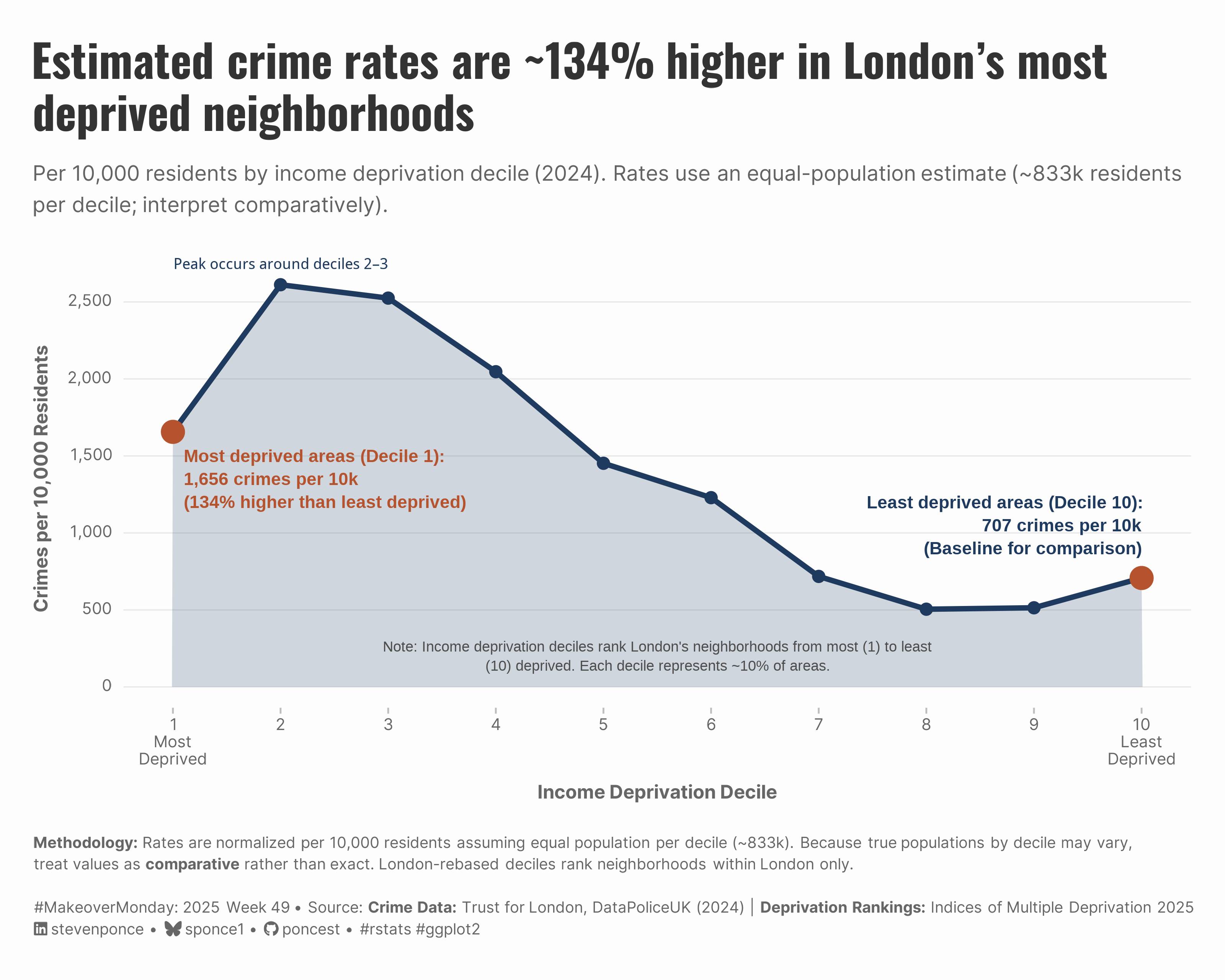
title: "Estimated crime rates are ~134% higher in London’s most<br>deprived neighborhoods"
subtitle: "Per 10,000 residents by income deprivation decile (2024). Rates use an equal-population estimate (~833k residents per decile; interpret comparatively)"
description: "Analyzing London's crime gradient across income deprivation levels using per capita rates. The visualization reveals that crime rates in the most deprived neighborhoods are ~134% higher than in the least deprived areas, even after population adjustment."
date: "2025-12-16"
author:
- name: "Steven Ponce"
url: "https://stevenponce.netlify.app"
citation:
url: "https://stevenponce.netlify.app/data_visualizations/MakeoverMonday/2025/mm_2025_49.html"
categories: ["MakeoverMonday", "2025"]
tags: [
"makeover-monday",
"london-crime",
"income-deprivation",
"per-capita-analysis",
"ggplot2",
"area-chart",
"gradient-visualization",
"population-adjustment",
"data-transparency",
"indices-of-deprivation",
"crime-statistics",
"inequality",
"uk-data",
"2025-week-49"
]
image: "thumbnails/mm_2025_49.png"
format:
html:
toc: true
toc-depth: 5
code-link: true
code-fold: true
code-tools: true
code-summary: "Show code"
editor_options:
chunk_output_type: inline
execute:
freeze: true
cache: true
error: false
message: false
warning: false
eval: true
---
```{r}
#| label: setup-links
#| include: false
# CENTRALIZED LINK MANAGEMENT
## Project-specific info
current_year <- 2025
current_week <- 49
project_file <- "mm_2025_49.qmd"
project_image <- "mm_2025_49.png"
## Data Sources
data_main <- "https://data.world/makeovermonday/2025w49-london-crimes-by-income-deprivation-decile"
data_secondary <- "https://data.world/makeovermonday/2025w49-london-crimes-by-income-deprivation-decile"
## Repository Links
repo_main <- "https://github.com/poncest/personal-website/"
repo_file <- paste0("https://github.com/poncest/personal-website/blob/master/data_visualizations/MakeoverMonday/", current_year, "/", project_file)
## External Resources/Images
chart_original <- "https://raw.githubusercontent.com/poncest/MakeoverMonday/refs/heads/master/2025/Week_48/original_chart.png"
## Organization/Platform Links
org_primary <- "https://trustforlondon.org.uk/data/crime-and-income-deprivation/"
org_secondary <- "https://trustforlondon.org.uk/data/crime-and-income-deprivation/"
# Helper function to create markdown links
create_link <- function(text, url) {
paste0("[", text, "](", url, ")")
}
# Helper function for citation-style links
create_citation_link <- function(text, url, title = NULL) {
if (is.null(title)) {
paste0("[", text, "](", url, ")")
} else {
paste0("[", text, "](", url, ' "', title, '")')
}
}
```
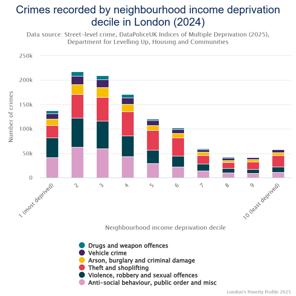
### Original
The original visualization comes from `r create_link("London crimes by income deprivation decile", data_secondary)`
### Makeover
{#fig-1}
### Methodology & Data Sources
#### Population Estimates & Per Capita Calculations
This analysis uses **per capita crime rates** (crimes per 10,000 residents) rather than raw counts to enable fair comparison across income deprivation deciles. Since population data aggregated by income deprivation decile was not readily available, we estimated populations based on:
- **London LSOA count:** 4,835 Lower Layer Super Output Areas ([London Datastore](https://data.london.gov.uk/dataset/lsoa-atlas-2n8zy/))
- **Average LSOA population:** 1,722 residents
- **Estimated population per decile:** \~833,000 residents (assuming roughly equal distribution)
- **Total estimated:** 8.33 million (vs. 8.9 million actual London population, 2021 Census)
**Note:** Trust for London uses London-rebased income deprivation deciles, ranking only London's 4,835 LSOAs into deciles (not England-wide rankings).
#### Critical Limitations & Assumptions
::: {.callout-warning collapse="false"}
##### Key Assumptions About Population Estimates
**1. Equal Distribution Assumption** - We assume approximately equal population across all 10 income deprivation deciles - Each decile: \~483-484 LSOAs × 1,722 residents = \~833,000 people - This is a **simplification** - actual populations likely vary by decile
**2. Why Estimates Were Necessary** - IoD2025 File 7 (official population denominators) was not accessible - No readily available population data aggregated by income deprivation decile - Per capita analysis requires population denominators for meaningful comparison
**3. Validity of Findings** - Under equal-population assumption: 134% difference persists (raw counts = per capita rates) - This suggests the crime disparity is **real**, not merely a population artifact - More deprived areas may have different population density than affluent areas
**4. Interpretation Guidance** - Per capita rates shown are based on **estimated**, not actual, populations - True rates may vary if actual population distribution differs significantly - **Treat values as comparative** rather than exact - All visualizations note this limitation in titles/subtitles/captions
:::
#### Data Preparation Pipeline
The CSV files used in this analysis were generated using a Python preprocessing script that calculated per capita crime rates with population estimates.
::: {.callout-note collapse="true"}
##### Reproducibility: Data Preparation Steps
**To reproduce the analysis from raw data:**
1. **Run the Python preprocessing script:**
- Script: [`mm_2025_week49_prep.py`](https://github.com/poncest/MakeoverMonday/blob/master/2025/Week_49/mm_2025_week49_prep.py)
- Input: `mom_week49_data.csv` (raw crime counts from [data.world](https://data.world/makeovermonday/2025w49-london-crimes-by-income-deprivation-decile))
- Output: Two tidy CSV files with per capita rates
2. **Run the R visualization script** (this document)
- Uses the pre-calculated per capita rates
- Creates the final visualization
**The Python script documents:** - Population estimation methodology (4,835 LSOAs × 1,722 avg residents) - Per capita rate calculations (crimes per 10,000 residents)\
- All assumptions and limitations (detailed above)
**Repository:** [MakeoverMonday/2025/Week_49](https://github.com/poncest/MakeoverMonday/tree/master/2025/Week_49)
:::
#### Data Sources
- **Crime Data:** Trust for London, DataPoliceUK (January-December 2024)
- **Deprivation Rankings:** [Indices of Multiple Deprivation 2025](https://www.gov.uk/government/statistics/english-indices-of-deprivation-2025) (IoD2025)
- **Population Reference:** [London Datastore - LSOA Atlas](https://data.london.gov.uk/dataset/lsoa-atlas-2n8zy/)
- **Challenge Data:** [data.world - MakeoverMonday Week 49](https://data.world/makeovermonday/2025w49-london-crimes-by-income-deprivation-decile)
### <mark> **Steps to Create this Graphic** </mark>
#### 1. Load Packages & Setup
```{r}
#| label: load
#| warning: false
#| message: false
#| results: "hide"

## 1. LOAD PACKAGES & SETUP ----
suppressPackageStartupMessages({
  if (!require("pacman")) install.packages("pacman")
  pacman::p_load(
  tidyverse,     # Easily Install and Load the 'Tidyverse'
  janitor,       # Simple Tools for Examining and Cleaning Dirty Data
  skimr,         # Compact and Flexible Summaries of Data
  scales,        # Scale Functions for Visualization
  ggtext,        # Improved Text Rendering Support for 'ggplot2'
  showtext,      # Using Fonts More Easily in R Graphs
  glue           # Interpreted String Literals
)
})

### |- figure size ----
camcorder::gg_record(
    dir    = here::here("temp_plots"),
    device = "png",
    width  = 10,
    height = 8,
    units  = "in",
    dpi    = 320
)

# Source utility functions
suppressMessages(source(here::here("R/utils/fonts.R")))
source(here::here("R/utils/social_icons.R"))
source(here::here("R/utils/image_utils.R"))
source(here::here("R/themes/base_theme.R"))
```
#### 2. Read in the Data
```{r}
#| label: read
#| include: true
#| eval: true
#| warning: false
#|

total_crimes_by_decile <- read_csv(
   here::here("data/MakeoverMonday/2025/london_total_crimes_by_deprivation.csv")) |>
  clean_names()
```
#### 3. Examine the Data
```{r}
#| label: examine
#| include: true
#| eval: true
#| results: 'hide'
#| warning: false

glimpse(total_crimes_by_decile)
skim(total_crimes_by_decile) |> summary()
```
#### 4. Tidy Data
```{r}
#| label: tidy
#| warning: false

### |-  data wrangling ----
# Baseline = least deprived (decile 10)
baseline_rate <- total_crimes_by_decile |>
  filter(decile_num == 10) |>
  pull(total_crimes_per_10k)

crime_gradient <- total_crimes_by_decile |>
  mutate(
    baseline_rate = baseline_rate,
    rate_ratio = total_crimes_per_10k / baseline_rate,
    pct_difference = ((total_crimes_per_10k - baseline_rate) / baseline_rate) * 100
  )

# Values for annotations
most_deprived_rate <- crime_gradient |> filter(decile_num == 1)  |> pull(total_crimes_per_10k)
least_deprived_rate <- crime_gradient |> filter(decile_num == 10) |> pull(total_crimes_per_10k)
overall_pct_diff <- crime_gradient |> filter(decile_num == 1) |> pull(pct_difference)

# Identify peak decile
peak_decile <- crime_gradient |>
  slice_max(total_crimes_per_10k, n = 1, with_ties = FALSE) |>
  pull(decile_num)

peak_rate <- crime_gradient |>
  filter(decile_num == peak_decile) |>
  pull(total_crimes_per_10k)
```
#### 5. Visualization Parameters
```{r}
#| label: params
#| include: true
#| warning: false

### |-  plot aesthetics ----
# Get base colors with custom palette
colors <- get_theme_colors(
  palette = list(
    col_primary = "#1E3A5F",
    col_danger  = "#B5532F"
  )
)

### |-  Main titles ----
title_text <- "Estimated crime rates are ~134% higher in London’s most<br>deprived neighborhoods"

subtitle_text <- str_glue(
  "Per 10,000 residents by income deprivation decile (2024). ",
  "Rates use an equal-population estimate (~833k residents<br>per decile; interpret comparatively). "
)

caption_text <- create_social_caption_02_mm(
  mm_year = 2025, mm_week = 49,
  source_text = str_glue(
    "**Crime Data:** Trust for London, DataPoliceUK (2024) | ",
    "**Deprivation Rankings:** Indices of Multiple Deprivation 2025<br>"
  ),
  note_text = str_glue(
    "**Methodology:** Rates are normalized per 10,000 residents assuming equal population per decile (~833k). ",
    "Because true populations by decile may vary,<br>treat values as **comparative** rather than exact. ",
    "London-rebased deciles rank neighborhoods within London only.<br>"
  )
)

### |-  fonts ----
setup_fonts()
fonts <- get_font_families()

### |-  plot theme ----

# Start with base theme
base_theme <- create_base_theme(colors)

# Add weekly-specific theme elements
weekly_theme <- extend_weekly_theme(
  base_theme,
  theme(
    # # Text styling
    plot.title = element_text(
      size = rel(1.5), family = fonts$title, face = "bold",
      color = colors$title, lineheight = 1.1, hjust = 0,
      margin = margin(t = 5, b = 10)
    ),
    plot.subtitle = element_markdown(
      size = rel(0.9), family = fonts$subtitle, face = "italic",
      color = alpha(colors$subtitle, 0.9), lineheight = 1.1,
      margin = margin(t = 0, b = 20)
    ),

    # Legend formatting
    legend.position = "plot",
    legend.justification = "right",
    legend.margin = margin(l = 12, b = 5),
    legend.key.size = unit(0.8, "cm"),
    legend.box.margin = margin(b = 10),

    # Axis formatting
    axis.ticks.y = element_blank(),
    axis.ticks.x = element_line(color = "gray", linewidth = 0.5),

    axis.title.x = element_text(
      face = "bold", size = rel(0.85),
      margin = margin(t = 10), family = fonts$subtitle,
      color = "gray40"
    ),
    axis.title.y = element_text(
      face = "bold", size = rel(0.85),
      margin = margin(r = 10), family = fonts$subtitle,
      color = "gray40"
    ),
    axis.text.x = element_text(
      size = rel(0.85), family = fonts$subtitle,
      color = "gray40"
    ),
    axis.text.y = element_markdown(
      size = rel(0.85), family = fonts$subtitle,
      color = "gray40"
    ),

    # Grid lines
    panel.grid.minor = element_line(color = "#ecf0f1", linewidth = 0.2),
    panel.grid.major = element_line(color = "#ecf0f1", linewidth = 0.4),

    # Margin
    plot.margin = margin(20, 20, 20, 20)
  )
)

# Set theme
theme_set(weekly_theme)
```
#### 6. Plot
```{r}
#| label: plot
#| warning: false

### |-  main plot ----
p <-
  ggplot(crime_gradient, aes(x = decile_num, y = total_crimes_per_10k)) +
  # Geoms
  geom_area(fill = colors$palette$col_primary, alpha = 0.20) +
  geom_line(color = colors$palette$col_primary, linewidth = 1.5) +
  geom_point(color = colors$palette$col_primary, size = 3) +
  geom_point(
    data = crime_gradient |> filter(decile_num %in% c(1, 10)),
    size = 6, color = colors$palette$col_danger
  ) +
  # Annotations
  annotate(
    "text",
    x = 1.1, y = 1350,
    label = glue(
      "Most deprived areas (Decile 1):\n",
      "{comma(round(most_deprived_rate))} crimes per 10k\n",
      "({round(overall_pct_diff)}% higher than least deprived)"
    ),
    size = 3.6, hjust = 0,
    fontface = "bold", lineheight = 1.1,
    color = colors$palette$col_danger
  ) +
  annotate(
    "text",
    x = 10.0, y = 1050,
    label = glue(
      "Least deprived areas (Decile 10):\n",
      "{comma(round(least_deprived_rate))} crimes per 10k\n",
      "(Baseline for comparison)"
    ),
    size = 3.6, hjust = 1,
    fontface = "bold", lineheight = 1.1,
    color = colors$palette$col_primary
  ) +
  annotate(
    "text",
    x = peak_decile, y = 2700,
    label = "Peak occurs around deciles 2–3",
    size = 3.2,
    fontface = "bold",
    color = colors$palette$col_primary,
    vjust = -0.2
  ) +
  annotate(
    "text",
    x = 5.5, y = 200,
    label = str_wrap(
      "Note: Income deprivation deciles rank London's neighborhoods from most (1) to least (10) deprived. Each decile represents ~10% of areas.",
      width = 86
    ),
    size = 3,
    color = "gray30",
    lineheight = 1.1,
    hjust = 0.5
  ) +
  # Scales
  scale_x_continuous(
    breaks = 1:10,
    labels = c(
      "1\nMost\nDeprived", "2", "3", "4", "5", "6", "7", "8", "9",
      "10\nLeast\nDeprived"
    )
  ) +
  scale_y_continuous(
    labels = comma,
    limits = c(0, 2700),
    breaks = seq(0, 2500, 500)
  ) +
  # Labs
  labs(
    title = title_text,
    subtitle = subtitle_text,
    caption = caption_text,
    x = "Income Deprivation Decile",
    y = "Crimes per 10,000 Residents"
  ) +
  # Theme
  theme(
    plot.title = element_markdown(
      size = rel(1.9),
      family = fonts$title,
      face = "bold",
      color = colors$title,
      lineheight = 1.15,
      margin = margin(t = 5, b = 10)
    ),
    plot.subtitle = element_markdown(
      size = rel(0.88),
      family = fonts$subtitle,
      color = alpha(colors$subtitle, 0.88),
      lineheight = 1.5,
      margin = margin(t = 5, b = 20)
    ),
    plot.caption = element_markdown(
      size = rel(0.65),
      family = fonts$subtitle,
      color = colors$caption,
      hjust = 0,
      lineheight = 1.4,
      margin = margin(t = 20, b = 5)
    ),
    panel.grid.minor.x = element_blank(),
    panel.grid.major.x = element_blank(),
    panel.grid.minor.y = element_blank(),
    panel.grid.major.y = element_line(color = "gray90", linewidth = 0.3),
  )
```
#### 7. Save
```{r}
#| label: save
#| warning: false

### |-  plot image ----
save_plot(
  plot = p,
  type = "makeovermonday",
  year = current_year,
  week = current_week,
  width = 10,
  height = 8
  )
```
#### 8. Session Info
::: {.callout-tip collapse="true"}
##### Expand for Session Info
```{r, echo = FALSE}
#| eval: true
#| warning: false
sessionInfo()
```
:::
#### 9. GitHub Repository
::: {.callout-tip collapse="true"}
##### Expand for GitHub Repo
The complete code for this analysis is available in `r create_link(project_file, repo_file)`.
For the full repository, `r create_link("click here", repo_main)`.
:::
#### 10. References
::: {.callout-tip collapse="true"}
##### Expand for References
1. Data:
- Makeover Monday `r current_year` Week `r current_week`: `r create_link("London crimes by income deprivation decile", data_main)`
2. Article
- `r create_link("London crimes by income deprivation decile", data_secondary)`
:::
#### 11. Custom Functions Documentation
::: {.callout-note collapse="true"}
##### 📦 Custom Helper Functions
This analysis uses custom functions from my personal module library for efficiency and consistency across projects.
**Functions Used:**
- **`fonts.R`**: `setup_fonts()`, `get_font_families()` - Font management with showtext
- **`social_icons.R`**: `create_social_caption()` - Generates formatted social media captions
- **`image_utils.R`**: `save_plot()` - Consistent plot saving with naming conventions
- **`base_theme.R`**: `create_base_theme()`, `extend_weekly_theme()`, `get_theme_colors()` - Custom ggplot2 themes
**Why custom functions?**\
These utilities standardize theming, fonts, and output across all my data visualizations. The core analysis (data tidying and visualization logic) uses only standard tidyverse packages.
**Source Code:**\
View all custom functions → [GitHub: R/utils](https://github.com/poncest/personal-website/tree/master/R)
:::

