---
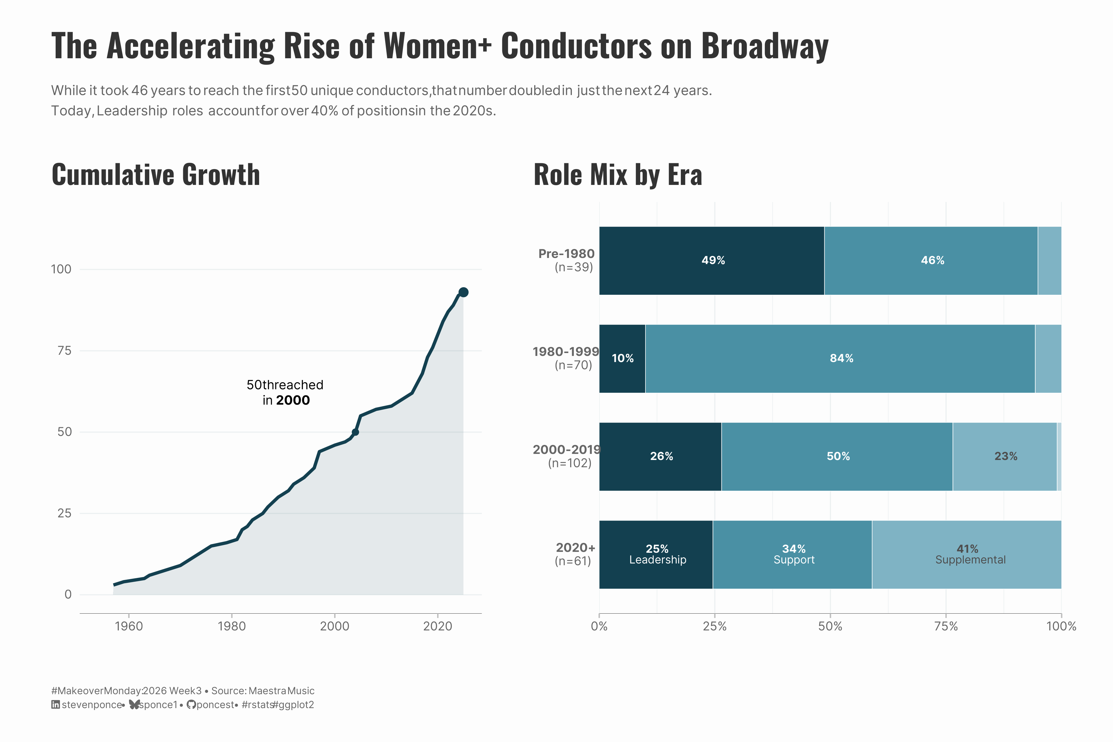
title: "The Accelerating Rise of Women+ Conductors on Broadway"
subtitle: "While it took 46 years to reach the first 50 unique conductors, that number doubled in just the next 24 years. Today, Leadership roles account for over 40% of positions in the 2020s."
description: "A two-panel visualization exploring the growth of women+ conductors on Broadway from 1954 to present. The analysis tracks both the accelerating cumulative count of unique conductors and the shifting distribution of role tiers—from Support-heavy in the 1980s-90s to Leadership-dominant in the 2020s. "
date: "2026-01-19"
author:
- name: "Steven Ponce"
url: "https://stevenponce.netlify.app"
citation:
url: "https://stevenponce.netlify.app/data_visualizations/MakeoverMonday/2026/mm_2026_03.html"
categories: ["MakeoverMonday", "2026"]
tags: [
"makeover-monday",
"data-visualization",
"ggplot2",
"patchwork",
"broadway",
"women-in-leadership",
"gender-equity",
"performing-arts",
"time-series",
"stacked-bar-chart",
"cumulative-analysis",
"maestra-music"
]
image: "thumbnails/mm_2026_03.png"
format:
html:
toc: true
toc-depth: 5
code-link: true
code-fold: true
code-tools: true
code-summary: "Show code"
editor_options:
chunk_output_type: inline
execute:
freeze: true
cache: true
error: false
message: false
warning: false
eval: true
---
```{r}
#| label: setup-links
#| include: false
# CENTRALIZED LINK MANAGEMENT
## Project-specific info
current_year <- 2026
current_week <- 03
project_file <- "mm_2026_03.qmd"
project_image <- "mm_2026_03.png"
## Data Sources
data_main <- "https://data.world/makeovermonday/2026w3-women-conductors-on-broadway"
data_secondary <- "https://data.world/makeovermonday/2026w3-women-conductors-on-broadway"
## Repository Links
repo_main <- "https://github.com/poncest/personal-website/"
repo_file <- paste0("https://github.com/poncest/personal-website/blob/master/data_visualizations/MakeoverMonday/", current_year, "/", project_file)
## External Resources/Images
chart_original <- "https://raw.githubusercontent.com/poncest/MakeoverMonday/refs/heads/master/2028/Week_02/original_chart.png"
## Organization/Platform Links
org_primary <- "https://maestramusic.org/resources/timelines/timeline-of-broadway-conductors-and-mds/"
org_secondary <- "https://maestramusic.org/resources/timelines/timeline-of-broadway-conductors-and-mds/"
# Helper function to create markdown links
create_link <- function(text, url) {
paste0("[", text, "](", url, ")")
}
# Helper function for citation-style links
create_citation_link <- function(text, url, title = NULL) {
if (is.null(title)) {
paste0("[", text, "](", url, ")")
} else {
paste0("[", text, "](", url, ' "', title, '")')
}
}
```
### Original
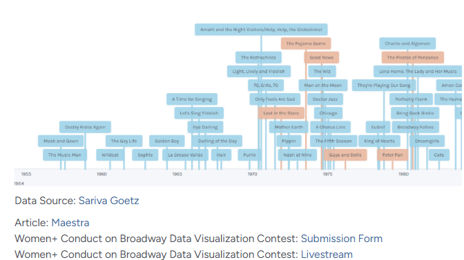
The original visualization comes from `r create_link("Women+ Conductors on Broadway", data_secondary)`
### Makeover
{#fig-1}
### [**Steps to Create this Graphic**]{.mark}
#### [1. Load Packages & Setup]{.smallcaps}
```{r}
#| label: load
#| warning: false
#| message: false
#| results: "hide"

## 1. LOAD PACKAGES & SETUP ----
suppressPackageStartupMessages({
  if (!require("pacman")) install.packages("pacman")
  pacman::p_load(
    tidyverse, ggtext, showtext, scales, glue, patchwork, janitor, readxl
)
})

### |- figure size ----
camcorder::gg_record(
    dir    = here::here("temp_plots"),
    device = "png",
    width  = 12,
    height = 8,
    units  = "in",
    dpi    = 320
)

# Source utility functions
suppressMessages(source(here::here("R/utils/fonts.R")))
source(here::here("R/utils/social_icons.R"))
source(here::here("R/utils/image_utils.R"))
source(here::here("R/themes/base_theme.R"))
```
#### [2. Read in the Data]{.smallcaps}
```{r}
#| label: read
#| include: true
#| eval: true
#| warning: false
#|

### |- Current data (2025) ----
conductor_raw <- readxl::read_excel(
   here::here("data/MakeoverMonday/2026/Conductor Timeline Data_Contest.xlsx")) |>
  clean_names()
```
#### [3. Examine the Data]{.smallcaps}
```{r}
#| label: examine
#| include: true
#| eval: true
#| results: 'hide'
#| warning: false

glimpse(conductor_raw)
skimr::skim(conductor_raw) |> summary()
```
#### [4. Tidy Data]{.smallcaps}
```{r}
#| label: tidy
#| warning: false

# Define role tiers
role_tiers <- tribble(
  ~role,                         ~tier,          ~tier_order,
  "Music Supervisor",            "Leadership",   1,
  "Music Director",              "Leadership",   1,
  "Conductor",                   "Leadership",   1,
  "Co-Music Director",           "Leadership",   1,
  "Co-Music Supervisor",         "Leadership",   1,
  "Associate Music Director",    "Support",      2,
  "Associate Music Supervisor",  "Support",      2,
  "Associate Conductor",         "Support",      2,
  "Resident Music Supervisor",   "Support",      2,
  "Assistant Music Director",    "Support",      2,
  "Assistant Conductor",         "Support",      2,
  "Alternate Conductor",         "Supplemental", 3,
  "Substitute Conductor",        "Supplemental", 3,
  "Children's Music Director",   "Specialized",  4
)

conductor_clean <- conductor_raw |>
  mutate(
    year = year(opening_date),
    era = case_when(
      year < 1980 ~ "Pre-1980",
      year >= 1980 & year < 2000 ~ "1980-1999",
      year >= 2000 & year < 2020 ~ "2000-2019",
      year >= 2020 ~ "2020+"
    )
  ) |>
  left_join(role_tiers, by = "role") |>
  filter(!is.na(era), !is.na(tier))

# Panel 1 Data: Cumulative
cumulative_data <- conductor_clean |>
  distinct(person_id, year) |>
  group_by(person_id) |>
  summarize(first_year = min(year), .groups = "drop") |>
  count(first_year) |>
  arrange(first_year) |>
  mutate(cumulative = cumsum(n))

latest_val <- filter(cumulative_data, first_year == max(first_year))

m50 <- filter(cumulative_data, cumulative >= 50) |> slice(1)

# Panel 2 Data: Role Stats with Chronological Ordering
role_era_stats <- conductor_clean |>
  group_by(era) |>
  mutate(era_n = n()) |>
  ungroup() |>
  mutate(era_label = glue("**{era}**<br>(n={era_n})")) |>
  mutate(era_label = fct_reorder(era_label, year, .desc = TRUE)) |>
  count(era_label, tier) |>
  group_by(era_label) |>
  mutate(pct = n / sum(n)) |>
  ungroup() |>
  mutate(tier = factor(tier, levels = rev(c("Leadership", "Support", "Supplemental", "Specialized"))))
```
#### [5. Visualization Parameters]{.smallcaps}
```{r}
#| label: params
#| include: true
#| warning: false

### |-  plot aesthetics ----
# Get base colors with custom palette
colors <- get_theme_colors(
  palette = list(
    leadership = "#134050",
    support = "#4A90A4",
    supplemental = "#7FB3C4",
    specialized = "#B8D4DE"
  )
)

tier_colors <- c(
  "Leadership" = colors$palette$leadership,
  "Support" = colors$palette$support,
  "Supplemental" = colors$palette$supplemental,
  "Specialized" = colors$palette$specialized
)

### |-  Main titles ----
title_text <- "The Accelerating Rise of Women+ Conductors on Broadway"

subtitle_text <- str_glue(
  "While it took 46 years to reach the first 50 unique conductors, that number doubled in just the next 24 years.<br>",
  "Today, **Leadership roles** account for over 40% of positions in the 2020s."
)

caption_text <- create_mm_caption(
  mm_year = 2026, mm_week = 03,
  source_text = str_glue(
    "Maestra Music"
  )
)

### |-  fonts ----
setup_fonts()
fonts <- get_font_families()

### |-  plot theme ----

# Start with base theme
base_theme <- create_base_theme(colors)

# Add weekly-specific theme elements
weekly_theme <- extend_weekly_theme(
  base_theme,
  theme(
    # # Text styling
    plot.title = element_text(
      size = rel(1.5), family = fonts$title, face = "bold",
      color = colors$title, lineheight = 1.1, hjust = 0,
      margin = margin(t = 5, b = 10)
    ),
    plot.subtitle = element_markdown(
      size = rel(0.9), family = fonts$subtitle, face = "italic",
      color = alpha(colors$subtitle, 0.9), lineheight = 1.1,
      margin = margin(t = 0, b = 20)
    ),

    # Legend formatting
    legend.position = "plot",
    legend.justification = "right",
    legend.margin = margin(l = 12, b = 5),
    legend.key.size = unit(0.8, "cm"),
    legend.box.margin = margin(b = 10),

    # Axis formatting
    axis.line.x = element_line(color = "#252525", linewidth = .1),
    axis.ticks.y = element_blank(),
    axis.ticks.x = element_line(color = "gray", linewidth = 0.5),
    axis.title.x = element_text(
      face = "bold", size = rel(0.85),
      margin = margin(t = 10), family = fonts$subtitle,
      color = "gray40"
    ),
    axis.title.y = element_text(
      face = "bold", size = rel(0.85),
      margin = margin(r = 10), family = fonts$subtitle,
      color = "gray40"
    ),
    axis.text.x = element_text(
      size = rel(0.85), family = fonts$subtitle,
      color = "gray40"
    ),
    axis.text.y = element_markdown(
      size = rel(0.85), family = fonts$subtitle,
      color = "gray40"
    ),

    # Grid lines
    panel.grid.minor = element_line(color = "#ecf0f1", linewidth = 0.2),
    panel.grid.major = element_line(color = "#ecf0f1", linewidth = 0.4),

    # Margin
    plot.margin = margin(20, 20, 20, 20)
  )
)

# Set theme
theme_set(weekly_theme)
```
#### [6. Plot]{.smallcaps}
```{r}
#| label: plot
#| warning: false

### |-  p1: cummulative growth ----
p1 <-
  ggplot(cumulative_data, aes(first_year, cumulative)) +
  # Geoms
  geom_area(fill = colors$palette$leadership, alpha = 0.1) +
  geom_line(color = colors$palette$leadership, linewidth = 1.2) +
  geom_point(data = m50, color = colors$palette$leadership, size = 2) +
  geom_point(data = latest_val, color = colors$palette$leadership, size = 3) +
  # Annotate
  annotate("richtext",
    x = 1990, y = 62, label = "50th reached<br>in **2000**",
    fill = NA, label.color = NA, family = fonts$text, size = 3.5
  ) +
  annotate("text",
    x = 2024, y = 108, label = "103 Unique\nConductors",
    fontface = "bold", color = colors$leadership, family = fonts$text, hjust = 1, lineheight = 0.9
  ) +
  # Scales
  scale_x_continuous(limits = c(1954, 2025), breaks = seq(1960, 2020, 20)) +
  scale_y_continuous(limits = c(0, 115), breaks = seq(0, 100, 25)) +
  # Labs
  labs(title = "Cumulative Growth", x = NULL, y = NULL) +
  # Theme
  theme(panel.grid.minor = element_blank(), panel.grid.major.x = element_blank())

### |-  p2: role mix ----
# label data
label_data <- role_era_stats |>
  arrange(era_label, desc(tier)) |>
  group_by(era_label) |>
  mutate(
    cumsum_pct = cumsum(pct),
    label_pos = cumsum_pct - pct / 2,
    # Color logic: Light bars get dark text
    label_col = if_else(tier %in% c("Specialized", "Supplemental"), colors$text, "white"),
    # Label logic: Direct legend for top bar, % only for others if > 7%
    display_label = case_when(
      str_detect(era_label, "2020") ~ glue("**{percent(pct, 1)}**<br>{tier}"),
      pct >= 0.08 ~ glue("**{percent(pct, 1)}**"),
      TRUE ~ ""
    )
  )

p2 <-
ggplot(role_era_stats, aes(era_label, pct, fill = tier)) +
  # Geoms
  geom_col(width = 0.7, color = "white", linewidth = 0.2) +
  geom_richtext(data = label_data,
                aes(y = label_pos, label = display_label, color = label_col),
                fill = NA, label.color = NA, family = fonts$text, size = 3, lineheight = 1) +
  # Scales
  scale_fill_manual(values = tier_colors) +
  scale_color_identity() +
  scale_y_continuous(labels = percent_format(), expand = c(0, 0)) +
  coord_flip() +
  # Labs
  labs(title = "Role Mix by Era", x = NULL, y = NULL) +
  # theme_minimal(base_family = fonts$text) +
  # Theme
  theme(
    legend.position = "none",
    panel.grid = element_blank(),
    axis.text.y = element_markdown(lineheight = 1.1)
    )

### |-  combined plot ----
combined_plot <- p1 + p2 +
  plot_layout(widths = c(1, 1.15)) +
  plot_annotation(
    title = title_text,
    subtitle = subtitle_text,
    caption = caption_text,
    theme = theme(
      plot.title = element_text(
        size = rel(1.8),
        family = fonts$title,
        face = "bold",
        color = colors$title,
        lineheight = 1.15,
        margin = margin(t = 5, b = 10)
      ),
      plot.subtitle = element_markdown(
        size = rel(0.75),
        family = fonts$subtitle,
        color = alpha(colors$subtitle, 0.88),
        lineheight = 1.5,
        margin = margin(t = 5, b = 10)
      ),
      plot.caption = element_markdown(
        size = rel(0.55),
        family = fonts$subtitle,
        color = colors$caption,
        hjust = 0,
        lineheight = 1.4,
        margin = margin(t = 20, b = 5)
      ),
    )
  )
```
#### [7. Save]{.smallcaps}
```{r}
#| label: save
#| warning: false

### |-  plot image ----
save_plot_patchwork(
  plot = combined_plot,
  type = "makeovermonday",
  year = current_year,
  week = current_week,
  width = 12,
  height = 8
  )
```
#### [8. Session Info]{.smallcaps}
::: {.callout-tip collapse="true"}
##### Expand for Session Info
```{r, echo = FALSE}
#| eval: true
#| warning: false
sessionInfo()
```
:::
#### [9. GitHub Repository]{.smallcaps}
::: {.callout-tip collapse="true"}
##### Expand for GitHub Repo
The complete code for this analysis is available in `r create_link(project_file, repo_file)`.
For the full repository, `r create_link("click here", repo_main)`.
:::
#### [10. References]{.smallcaps}
::: {.callout-tip collapse="true"}
##### Expand for References
1. Data:
- Makeover Monday `r current_year` Week `r current_week`: `r create_link("Women+ Conductors on Broadway", data_main)`
2. Article
- `r create_link("Women+ Conductors on Broadway", data_secondary)`
:::
#### [11. Custom Functions Documentation]{.smallcaps}
::: {.callout-note collapse="true"}
##### 📦 Custom Helper Functions
This analysis uses custom functions from my personal module library for efficiency and consistency across projects.
**Functions Used:**
- **`fonts.R`**: `setup_fonts()`, `get_font_families()` - Font management with showtext
- **`social_icons.R`**: `create_social_caption()` - Generates formatted social media captions
- **`image_utils.R`**: `save_plot()` - Consistent plot saving with naming conventions
- **`base_theme.R`**: `create_base_theme()`, `extend_weekly_theme()`, `get_theme_colors()` - Custom ggplot2 themes
**Why custom functions?**\
These utilities standardize theming, fonts, and output across all my data visualizations. The core analysis (data tidying and visualization logic) uses only standard tidyverse packages.
**Source Code:**\
View all custom functions → [GitHub: R/utils](https://github.com/poncest/personal-website/tree/master/R)
:::

