---
title: "25 Years of Currency Shifts"
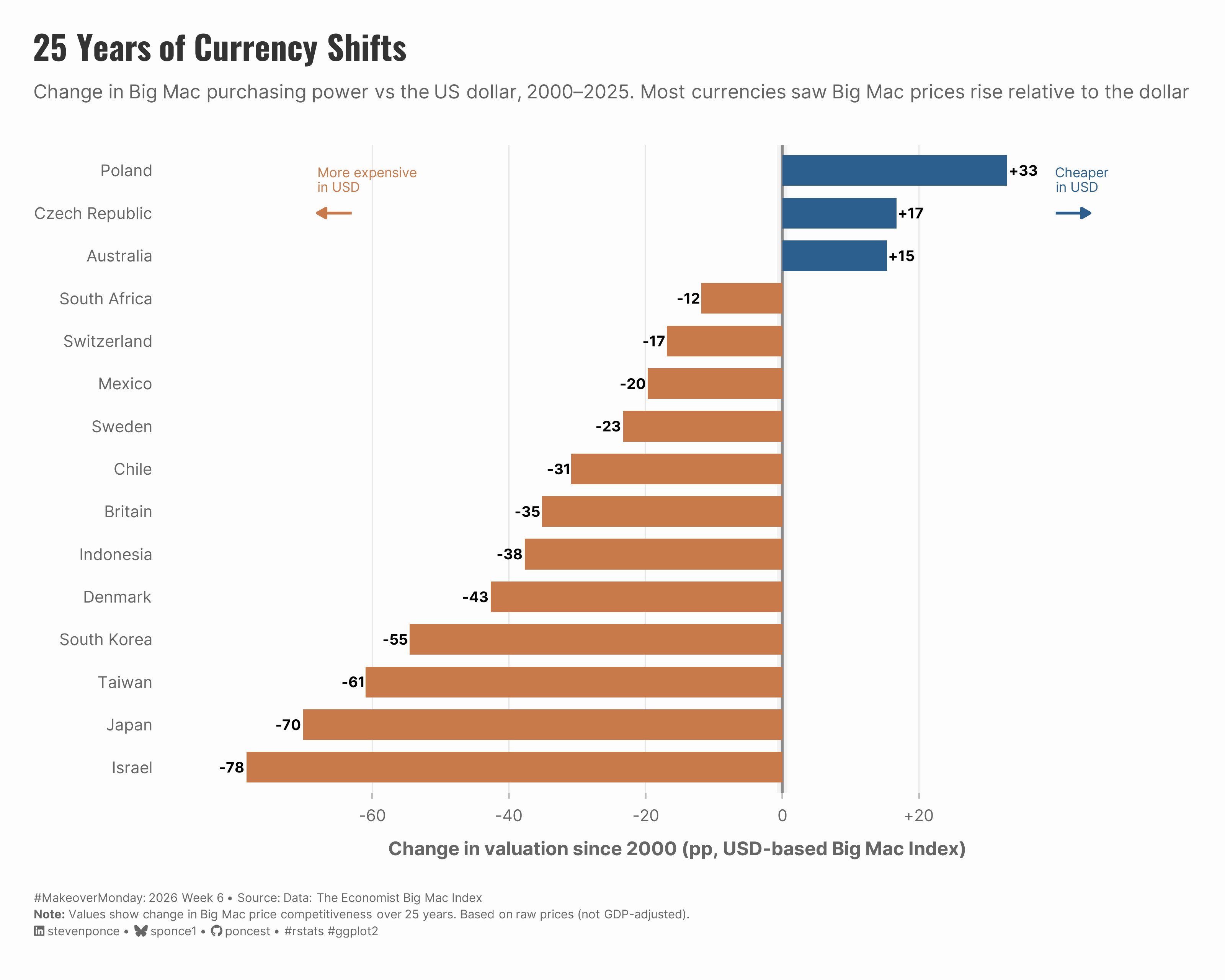
subtitle: "Change in Big Mac purchasing power vs the US dollar, 2000–2025. Most currencies saw Big Mac prices rise relative to the dollar"
description: "A makeover of The Economist's Big Mac Index reveals how purchasing power shifted against the US dollar from 2000 to 2025. This diverging bar chart shows 12 of 15 currencies weakened significantly—Israel, Japan, and Taiwan lost over 60 percentage points—while only Poland, Czech Republic, and Australia strengthened. Built with R and ggplot2, using semantic color choice and directional arrows for clarity."
date: "2026-02-10"
author:
- name: "Steven Ponce"
url: "https://stevenponce.netlify.app"
citation:
url: "https://stevenponce.netlify.app/data_visualizations/MakeoverMonday/2026/mm_2026_06.html"
categories: ["MakeoverMonday", "2026"]
tags: [
"makeover-monday",
"data-visualization",
"ggplot2",
"economics",
"currency",
"big-mac-index",
"purchasing-power-parity",
"diverging-bar-chart",
"the-economist",
"r-programming",
"financial-data",
"international-economics",
"exchange-rates",
"data-storytelling"
]
image: "thumbnails/mm_2026_06.png"
format:
html:
toc: true
toc-depth: 5
code-link: true
code-fold: true
code-tools: true
code-summary: "Show code"
editor_options:
chunk_output_type: inline
execute:
freeze: true
cache: true
error: false
message: false
warning: false
eval: true
---
```{r}
#| label: setup-links
#| include: false
# CENTRALIZED LINK MANAGEMENT
## Project-specific info
current_year <- 2026
current_week <- 06
project_file <- "mm_2026_06.qmd"
project_image <- "mm_2026_06.png"
## Data Sources
data_main <- "https://data.world/makeovermonday/2026w6-global-big-mac-index"
data_secondary <- "https://data.world/makeovermonday/2026w6-global-big-mac-index"
## Repository Links
repo_main <- "https://github.com/poncest/personal-website/"
repo_file <- paste0("https://github.com/poncest/personal-website/blob/master/data_visualizations/MakeoverMonday/", current_year, "/", project_file)
## External Resources/Images
chart_original <- "https://raw.githubusercontent.com/poncest/MakeoverMonday/refs/heads/master/2026/Week_06/original_chart.png"
## Organization/Platform Links
org_primary <- "https://www.economist.com/interactive/big-mac-index"
org_secondary <- "https://www.economist.com/interactive/big-mac-index"
# Helper function to create markdown links
create_link <- function(text, url) {
paste0("[", text, "](", url, ")")
}
# Helper function for citation-style links
create_citation_link <- function(text, url, title = NULL) {
if (is.null(title)) {
paste0("[", text, "](", url, ")")
} else {
paste0("[", text, "](", url, ' "', title, '")')
}
}
```
### Original
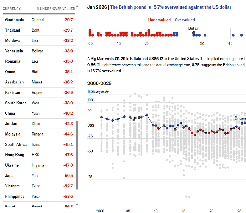
The original visualization comes from `r create_link("Global Big Mac Index", data_secondary)`
### Makeover
{#fig-1}
### [**Steps to Create this Graphic**]{.mark}
#### [1. Load Packages & Setup]{.smallcaps}
```{r}
#| label: load
#| warning: false
#| message: false
#| results: "hide"

## 1. LOAD PACKAGES & SETUP ----
suppressPackageStartupMessages({
  if (!require("pacman")) install.packages("pacman")
  pacman::p_load(
    tidyverse, ggtext, showtext, scales, glue,
    janitor, lubridate
)
})

### |- figure size ----
# camcorder::gg_record(
#     dir    = here::here("temp_plots"),
#     device = "png",
#     width  = 10,
#     height = 8,
#     units  = "in",
#     dpi    = 320
# )

# Source utility functions
suppressMessages(source(here::here("R/utils/fonts.R")))
source(here::here("R/utils/social_icons.R"))
source(here::here("R/utils/image_utils.R"))
source(here::here("R/themes/base_theme.R"))
```
#### [2. Read in the Data]{.smallcaps}
```{r}
#| label: read
#| include: true
#| eval: true
#| warning: false
#|

big_mac_index_raw <- read_csv(
  here::here("data/MakeoverMonday/2026/big-mac-full-index.csv")) |>
  clean_names()
```
#### [3. Examine the Data]{.smallcaps}
```{r}
#| label: examine
#| include: true
#| eval: true
#| results: 'hide'
#| warning: false

glimpse(big_mac_index_raw)
```
#### [4. Tidy Data]{.smallcaps}
```{r}
#| label: tidy
#| warning: false

### |-  prepare data ----
time_series_data <- big_mac_index_raw |>
  mutate(date = mdy(date))

latest_date <- max(time_series_data$date, na.rm = TRUE)

current_data <- time_series_data |>
  filter(date == latest_date) |>
  arrange(desc(usd_raw))

### |-  calculate 25-year change ----
first_obs <- time_series_data |>
  filter(year(date) == 2000) |>
  group_by(name) |>
  slice_min(date, n = 1, with_ties = FALSE) |>
  ungroup() |>
  select(name, usd_raw_start = usd_raw)

# Compute movers from 2000
currency_movers <- current_data |>
  inner_join(first_obs, by = "name") |>
  mutate(
    total_change = (usd_raw - usd_raw_start) * 100,
    direction = if_else(total_change > 0, "Strengthened", "Weakened")
  ) |>
  slice_max(order_by = abs(total_change), n = 15, with_ties = FALSE) |>
  arrange(total_change) |>
  mutate(name = fct_inorder(name))
```
#### [5. Visualization Parameters]{.smallcaps}
```{r}
#| label: params
#| include: true
#| warning: false

### |-  plot aesthetics ----
colors <- get_theme_colors(
  palette = list(
    strengthened  = "#2C5F8D",
    weakened      = "#C97A4A",
    neutral_dark  = "#5378A6",
    neutral_light = "gray90"
  )
)

### |-  Main titles ----
title_text <- "25 Years of Currency Shifts"

subtitle_text <- str_glue(
  "Change in Big Mac purchasing power vs the US dollar, 2000–2025. Most currencies saw Big Mac prices rise relative to the dollar"
)

caption_text <- create_mm_caption(
  mm_year = 2026, mm_week = 06,
  source_text = "Data: The Economist Big Mac Index<br>**Note:** Values show change in Big Mac price competitiveness over 25 years. Based on raw prices (not GDP-adjusted)."
)

### |-  fonts ----
setup_fonts()
fonts <- get_font_families()

### |-  plot theme ----

# Start with base theme
base_theme <- create_base_theme(colors)

# Add weekly-specific theme elements
weekly_theme <- extend_weekly_theme(
  base_theme,
  theme(
    # # Text styling
    plot.title = element_text(
      size = rel(1.3), family = fonts$title, face = "bold",
      color = colors$title, lineheight = 1.1, hjust = 0,
      margin = margin(t = 5, b = 10)
    ),
    plot.subtitle = element_text(
      size = rel(0.8), family = fonts$subtitle, face = "italic",
      color = alpha(colors$subtitle, 0.9), lineheight = 1.1,
      margin = margin(t = 0, b = 20)
    ),

    # Legend formatting
    legend.position = "plot",
    legend.justification = "right",
    legend.margin = margin(l = 12, b = 5),
    legend.key.size = unit(0.8, "cm"),
    legend.box.margin = margin(b = 10),

    # Axis formatting
    # axis.line.x = element_line(color = "#252525", linewidth = .1),
    # axis.ticks.y = element_blank(),
    axis.ticks.x = element_line(color = "gray", linewidth = 0.5),
    axis.title.x = element_text(
      face = "bold", size = rel(0.85),
      margin = margin(t = 10), family = fonts$subtitle,
      color = "gray40"
    ),
    axis.title.y = element_text(
      face = "bold", size = rel(0.85),
      margin = margin(r = 10), family = fonts$subtitle,
      color = "gray40"
    ),
    axis.text.x = element_text(
      size = rel(0.85), family = fonts$subtitle,
      color = "gray40"
    ),
    axis.text.y = element_markdown(
      size = rel(0.85), family = fonts$subtitle,
      color = "gray40"
    ),

    # Grid lines
    panel.grid.minor = element_line(color = "#ecf0f1", linewidth = 0.2),
    panel.grid.major = element_line(color = "#ecf0f1", linewidth = 0.4),

    # Margin
    plot.margin = margin(20, 20, 20, 20)
  )
)

# Set theme
theme_set(weekly_theme)
```
#### [6. Plot]{.smallcaps}
```{r}
#| label: plot
#| warning: false

### |- final plot ----
p <- ggplot(currency_movers, aes(x = total_change, y = name)) +
  # Annotate
  annotate(
    "rect",
    xmin = -0.75, xmax = 0.75,
    ymin = -Inf, ymax = Inf,
    fill = "gray95", alpha = 1
  ) +
  # Geoms
  geom_vline(xintercept = 0, linewidth = 0.8, color = "gray55") +
  geom_col(aes(fill = direction), width = 0.72, show.legend = FALSE) +
  geom_text(
    aes(
      label = sprintf("%+.0f", total_change),
      hjust = if_else(total_change >= 0, -0.10, 1.10)
    ),
    size = 3,
    fontface = "bold"
  ) +
  # Annotate
  annotate(
    "segment",
    x = -63, xend = -68,
    y = 14, yend = 14,
    arrow = arrow(length = unit(0.2, "cm"), type = "closed"),
    color = colors$palette$weakened,
    linewidth = 0.8
  ) +
  annotate(
    "text",
    x = -68, y = 14.5,
    label = "More expensive\nin USD",
    hjust = 0,
    vjust = 0,
    size = 2.8,
    color = colors$palette$weakened,
    fontface = "italic",
    lineheight = 0.9
  ) +
  annotate(
    "segment",
    x = 40, xend = 45,
    y = 14, yend = 14,
    arrow = arrow(length = unit(0.2, "cm"), type = "closed"),
    color = colors$palette$strengthened,
    linewidth = 0.8
  ) +
  annotate(
    "text",
    x = 40, y = 14.5,
    label = "Cheaper\nin USD",
    hjust = 0,
    vjust = 0,
    size = 2.8,
    color = colors$palette$strengthened,
    fontface = "italic",
    lineheight = 0.9
  ) +
  # Scales
  scale_fill_manual(values = c(
    "Strengthened" = colors$palette$strengthened,
    "Weakened" = colors$palette$weakened
  )) +
  scale_x_continuous(
    labels = label_number(style_positive = "plus"),
    expand = expansion(mult = c(0.10, 0.12)),
    breaks = seq(-60, 30, by = 20)
  ) +
  coord_cartesian(clip = "off") +
  # Labs
  labs(
    title = title_text,
    subtitle = subtitle_text,
    caption = caption_text,
    x = "Change in valuation since 2000 (pp, USD-based Big Mac Index)",
    y = NULL
  ) +
  # Theme
  theme(
    panel.grid.minor = element_blank(),
    panel.grid.major.y = element_blank(),
    panel.grid.major.x = element_line(color = "gray90", linewidth = 0.3),
    plot.title = element_markdown(
      size = rel(1.4),
      family = fonts$title,
      face = "bold",
      color = colors$title,
      lineheight = 1.15,
      margin = margin(t = 0, b = 5)
    ),
    plot.subtitle = element_markdown(
      size = rel(0.8),
      family = fonts$subtitle,
      face = "italic",
      color = alpha(colors$subtitle, 0.88),
      lineheight = 1.5,
      margin = margin(t = 5, b = 25)
    ),
    plot.caption = element_markdown(
      size = rel(0.5),
      family = fonts$subtitle,
      color = colors$caption,
      hjust = 0,
      lineheight = 1.4,
      margin = margin(t = 20, b = 5)
    )
  )
```
#### [7. Save]{.smallcaps}
```{r}
#| label: save
#| warning: false

### |-  plot image ----
save_plot(
  plot = p,
  type = "makeovermonday",
  year = current_year,
  week = current_week,
  width = 10,
  height = 8
  )
```
#### [8. Session Info]{.smallcaps}
::: {.callout-tip collapse="true"}
##### Expand for Session Info
```{r, echo = FALSE}
#| eval: true
#| warning: false
sessionInfo()
```
:::
#### [9. GitHub Repository]{.smallcaps}
::: {.callout-tip collapse="true"}
##### Expand for GitHub Repo
The complete code for this analysis is available in `r create_link(project_file, repo_file)`.
For the full repository, `r create_link("click here", repo_main)`.
:::
#### [10. References]{.smallcaps}
::: {.callout-tip collapse="true"}
##### Expand for References
**Primary Data (Makeover Monday):**
1. Makeover Monday `r current_year` Week `r current_week`: `r create_link("Big Mac Index", data_main)`
2. Original Article: `r create_link("The Big Mac Index", "https://www.economist.com/interactive/big-mac-index")`
- Source: The Economist
- Coverage: Big Mac prices and currency valuations, 2000–2025
**Source Data:**
3. Big Mac Index Full Dataset: `r create_link("GitHub Repository", "https://github.com/TheEconomist/big-mac-data")`
- Source: The Economist
- Data includes: Raw and GDP-adjusted indices
- Big Mac prices from: McDonald's directly and reporting worldwide
- Exchange rates from: Refinitiv Datastream (July 2022 onwards)
- GDP data from: IMF World Economic Outlook reports
- Citation: The Economist. (2025). *Big Mac Index Data*. Retrieved from https://github.com/TheEconomist/big-mac-data
**Methodology References:**
4. The Economist's Big Mac Index Methodology: `r create_link("README Documentation", "https://github.com/TheEconomist/big-mac-data?tab=readme-ov-file")`
- Explains raw vs GDP-adjusted calculations
- Details data sources and collection methods
- Last updated: July 2022 methodology revision
**Note:** This visualization uses the **raw index** (not GDP-adjusted) to show changes in actual purchasing power of Big Macs across currencies from 2000 to 2025.
:::
#### [11. Custom Functions Documentation]{.smallcaps}
::: {.callout-note collapse="true"}
##### 📦 Custom Helper Functions
This analysis uses custom functions from my personal module library for efficiency and consistency across projects.
**Functions Used:**
- **`fonts.R`**: `setup_fonts()`, `get_font_families()` - Font management with showtext
- **`social_icons.R`**: `create_social_caption()` - Generates formatted social media captions
- **`image_utils.R`**: `save_plot()` - Consistent plot saving with naming conventions
- **`base_theme.R`**: `create_base_theme()`, `extend_weekly_theme()`, `get_theme_colors()` - Custom ggplot2 themes
**Why custom functions?**\
These utilities standardize theming, fonts, and output across all my data visualizations. The core analysis (data tidying and visualization logic) uses only standard tidyverse packages.
**Source Code:**\
View all custom functions → [GitHub: R/utils](https://github.com/poncest/personal-website/tree/master/R)
:::

