---
title: "Wildlife Loss Since 1970 Is Uneven — and Extreme in Freshwater Systems"
subtitle: ""
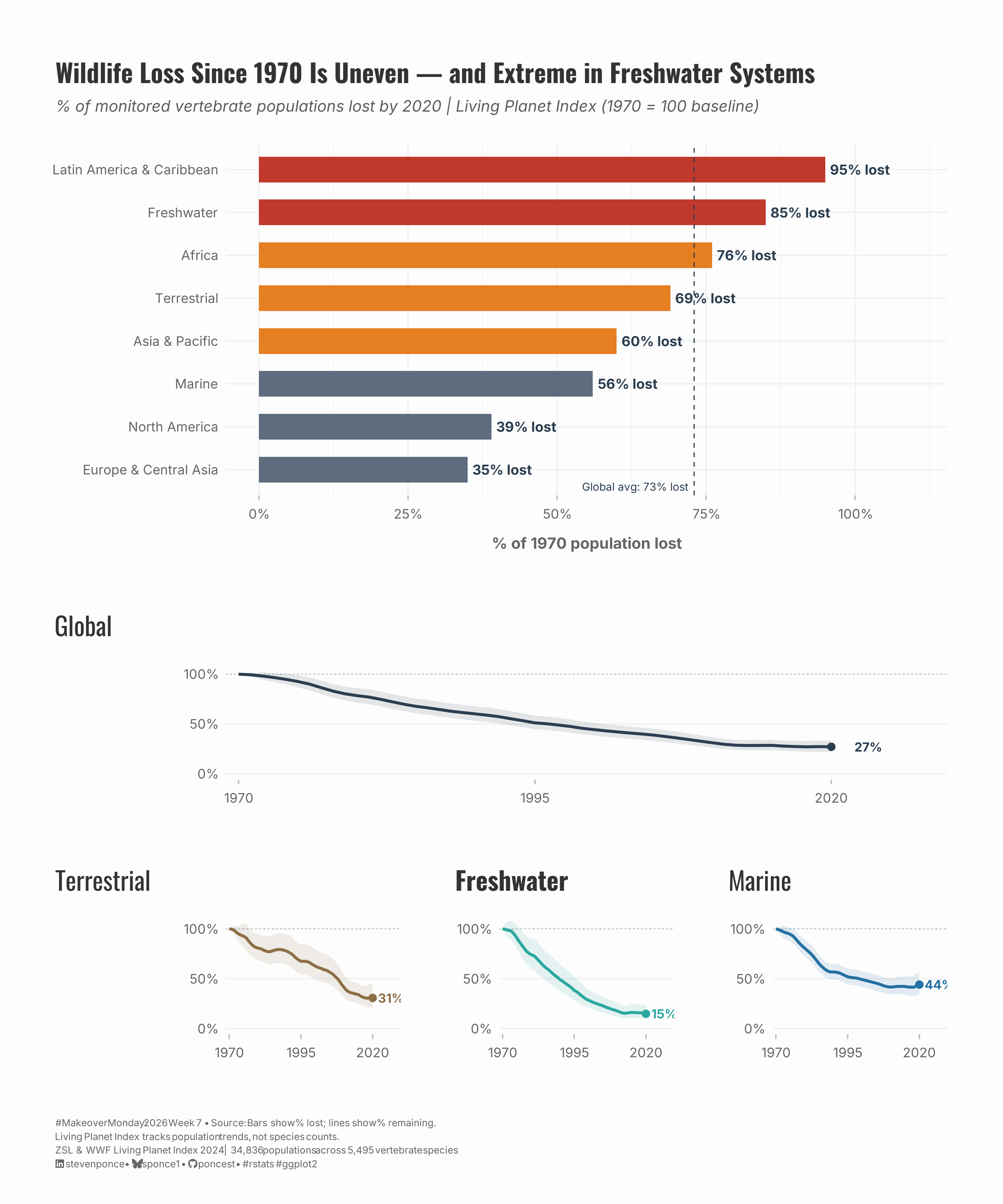
description: "A Makeover Monday visualization redesigning the Living Planet Index chart from ZSL & WWF. The makeover reframes the data as percentage lost, ranks all eight categories by severity, and reveals freshwater ecosystems as the primary driver of the most extreme regional declines."
date: "2026-02-16"
author:
- name: "Steven Ponce"
url: "https://stevenponce.netlify.app"
citation:
url: "https://stevenponce.netlify.app/data_visualizations/MakeoverMonday/2026/mm_2026_07.html"
categories: ["MakeoverMonday", "2026"]
tags: [
"makeover-monday",
"data-visualization",
"ggplot2",
"biodiversity",
"living-planet-index",
"wildlife-decline",
"freshwater",
"patchwork",
"bar-chart",
"line-chart",
"small-multiples",
"environmental-data",
"ZSL-WWF"
]
image: "thumbnails/mm_2026_07.png"
format:
html:
toc: true
toc-depth: 5
code-link: true
code-fold: true
code-tools: true
code-summary: "Show code"
editor_options:
chunk_output_type: inline
execute:
freeze: true
cache: true
error: false
message: false
warning: false
eval: true
---
```{r}
#| label: setup-links
#| include: false
# CENTRALIZED LINK MANAGEMENT
## Project-specific info
current_year <- 2026
current_week <- 07
project_file <- "mm_2026_07.qmd"
project_image <- "mm_2026_07.png"
## Data Sources
data_main <- "https://data.world/makeovermonday/2026w7-living-planet-index"
data_secondary <- "https://data.world/makeovermonday/2026w7-living-planet-index"
## Repository Links
repo_main <- "https://github.com/poncest/personal-website/"
repo_file <- paste0("https://github.com/poncest/personal-website/blob/master/data_visualizations/MakeoverMonday/", current_year, "/", project_file)
## External Resources/Images
chart_original <- "https://raw.githubusercontent.com/poncest/MakeoverMonday/refs/heads/master/2026/Week_07/original_chart.png"
## Organization/Platform Links
org_primary <- "https://livingplanet.panda.org/en-GB/"
org_secondary <- "https://livingplanet.panda.org/en-GB/"
# Helper function to create markdown links
create_link <- function(text, url) {
paste0("[", text, "](", url, ")")
}
# Helper function for citation-style links
create_citation_link <- function(text, url, title = NULL) {
if (is.null(title)) {
paste0("[", text, "](", url, ")")
} else {
paste0("[", text, "](", url, ' "', title, '")')
}
}
```
### Original
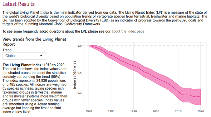
The original visualization comes from `r create_link("Living Planet Index", data_secondary)`
### Makeover
{#fig-1}
### [**Steps to Create this Graphic**]{.mark}
#### [1. Load Packages & Setup]{.smallcaps}
```{r}
#| label: load
#| warning: false
#| message: false
#| results: "hide"

## 1. LOAD PACKAGES & SETUP ----
suppressPackageStartupMessages({
  if (!require("pacman")) install.packages("pacman")
  pacman::p_load(
    tidyverse, ggtext, showtext, scales, glue,
  janitor, lubridate, patchwork
)
})

### |- figure size ----
camcorder::gg_record(
  dir    = here::here("temp_plots"),
  device = "png",
  width  = 10,
  height = 12,
  units  = "in",
  dpi    = 320
)

# Source utility functions
suppressMessages(source(here::here("R/utils/fonts.R")))
source(here::here("R/utils/social_icons.R"))
source(here::here("R/utils/image_utils.R"))
source(here::here("R/themes/base_theme.R"))
```
#### [2. Read in the Data]{.smallcaps}
```{r}
#| label: read
#| include: true
#| eval: true
#| warning: false
#|

lpi_raw <- readxl::read_excel(
  here::here("data/MakeoverMonday/2026/LPI 2024.xlsx")) |>
  clean_names()
```
#### [3. Examine the Data]{.smallcaps}
```{r}
#| label: examine
#| include: true
#| eval: true
#| results: 'hide'
#| warning: false

glimpse(lpi_raw)
```
#### [4. Tidy Data]{.smallcaps}
```{r}
#| label: tidy
#| warning: false

### |-  prepare data ----
lpi_data <- lpi_raw |>
  mutate(
    category = str_trim(category),
    lpi_pct = lpi_final * 100,
    ci_low = ci_low * 100,
    ci_high = ci_high * 100,
    category_label = case_when(
      category == "Europe and Central Asia" ~ "Europe & Central Asia",
      category == "Latin Amercia & Caribbean" ~ "Latin America & Caribbean",
      TRUE ~ category
    )
  )

endpoints <- lpi_data |>
  filter(year == 2020) |>
  mutate(
    pct_remaining = round(lpi_pct),
    pct_lost = round(100 - lpi_pct)
  )

global_end <- endpoints |> filter(category == "Global")
```
#### [5. Visualization Parameters]{.smallcaps}
```{r}
#| label: params
#| include: true
#| warning: false

### |-  plot aesthetics ----
colors <- get_theme_colors(
  palette = list(
    danger        = "#C0392B",
    primary       = "#2C3E50",
    freshwater    = "#2BA8A0",
    terrestrial   = "#8E6F47",
    marine        = "#2471A3",
    neutral_dark  = "#5D6D7E",
    neutral_mid   = "#AEB6BF",
    highlight     = "#E67E22"
  )
)

### |-  Main titles ----
title_text <- NULL

subtitle_text <- NULL

caption_text <- create_mm_caption(
  mm_year = 2026, mm_week = 07,
  source_text = glue(
    "Bars show % lost; lines show % remaining.<br>",
    "Living Planet Index tracks population trends, not species counts.<br>",
    "ZSL & WWF Living Planet Index 2024 | ",
    "34,836 populations across 5,495 vertebrate species"
  )
)

### |-  fonts ----
setup_fonts()
fonts <- get_font_families()

### |-  plot theme ----

# Start with base theme
base_theme <- create_base_theme(colors)

# Add weekly-specific theme elements
weekly_theme <- extend_weekly_theme(
  base_theme,
  theme(
    # # Text styling
    plot.title = element_text(
      size = rel(1.3), family = fonts$title, face = "bold",
      color = colors$title, lineheight = 1.1, hjust = 0,
      margin = margin(t = 5, b = 10)
    ),
    plot.subtitle = element_text(
      size = rel(0.8), family = fonts$subtitle, face = "italic",
      color = alpha(colors$subtitle, 0.9), lineheight = 1.1,
      margin = margin(t = 0, b = 20)
    ),

    # Legend formatting
    legend.position = "plot",
    legend.justification = "right",
    legend.margin = margin(l = 12, b = 5),
    legend.key.size = unit(0.8, "cm"),
    legend.box.margin = margin(b = 10),

    # Axis formatting
    # axis.line.x = element_line(color = "#252525", linewidth = .1),
    # axis.ticks.y = element_blank(),
    axis.ticks.x = element_line(color = "gray", linewidth = 0.5),
    axis.title.x = element_text(
      face = "bold", size = rel(0.85),
      margin = margin(t = 10), family = fonts$subtitle,
      color = "gray40"
    ),
    axis.title.y = element_text(
      face = "bold", size = rel(0.85),
      margin = margin(r = 10), family = fonts$subtitle,
      color = "gray40"
    ),
    axis.text.x = element_text(
      size = rel(0.85), family = fonts$subtitle,
      color = "gray40"
    ),
    axis.text.y = element_markdown(
      size = rel(0.85), family = fonts$subtitle,
      color = "gray40"
    ),

    # Grid lines
    panel.grid.minor = element_line(color = "#ecf0f1", linewidth = 0.2),
    panel.grid.major = element_line(color = "#ecf0f1", linewidth = 0.4),

    # Margin
    plot.margin = margin(20, 20, 20, 20)
  )
)

# Set theme
theme_set(weekly_theme)
```
#### [6. Plot]{.smallcaps}
```{r}
#| label: plot
#| warning: false

### |- PANEL 1 — DAMAGE REPORT (% LOST) ----

bars <- endpoints |>
  filter(category != "Global") |>
  mutate(
    category_label = fct_reorder(category_label, pct_lost),
    bar_color = case_when(
      pct_lost >= 80 ~ colors$palette$danger,
      pct_lost >= 60 ~ colors$palette$highlight,
      TRUE ~ colors$palette$neutral_dark
    )
  )

p1 <- ggplot(bars, aes(pct_lost, category_label)) +
  # Geoms
  geom_col(aes(fill = bar_color), width = 0.6) +
  geom_text(
    aes(label = paste0(pct_lost, "% lost")),
    hjust = -0.08,
    size = 3.5,
    fontface = "bold",
    family = fonts$text,
    color = colors$palette$primary
  ) +
  geom_vline(
    xintercept = global_end$pct_lost,
    linetype = "dashed",
    linewidth = 0.4,
    color = colors$palette$primary
  ) +
  annotate(
    "text",
    x = global_end$pct_lost - 1,
    y = 0.6,
    label = glue("Global avg: {global_end$pct_lost}% lost"),
    hjust = 1,
    size = 2.8,
    family = fonts$text,
    color = colors$palette$primary
  ) +
  # Scales
  scale_fill_identity() +
  scale_x_continuous(
    limits = c(0, 110),
    breaks = seq(0, 100, 25),
    labels = ~ paste0(.x, "%")
  ) +
  # Labs
  labs(
    title = "Wildlife Loss Since 1970 Is Uneven — and Extreme in Freshwater Systems",
    subtitle = glue(
      "% of monitored vertebrate populations lost by 2020 | ",
      "Living Planet Index (1970 = 100 baseline)"
    ),
    x = "% of 1970 population lost",
    y = NULL
  )

### |- PANEL 2 — ECOSYSTEM TRENDS (% REMAINING) ----
make_panel <- function(cat, col, bold = FALSE) {
  d <- lpi_data |> filter(category == cat)
  ep <- endpoints |> filter(category == cat)

  ggplot(d, aes(year)) +
    # Geoms
    geom_ribbon(aes(ymin = ci_low, ymax = ci_high),
      fill = col, alpha = 0.12
    ) +
    geom_hline(
      yintercept = 100, linetype = "dotted",
      color = colors$palette$neutral_dark, linewidth = 0.2
    ) +
    geom_line(aes(y = lpi_pct), color = col, linewidth = 1) +
    geom_point(
      data = d |> filter(year == 2020),
      aes(y = lpi_pct),
      color = col,
      size = 2
    ) +
    annotate(
      "text",
      x = 2022,
      y = ep$lpi_pct,
      label = paste0(ep$pct_remaining, "%"),
      hjust = 0,
      size = 3.2,
      fontface = "bold",
      family = fonts$text,
      color = col
    ) +
    # Scales
    scale_y_continuous(
      limits = c(0, 115),
      breaks = c(0, 50, 100),
      labels = ~ paste0(.x, "%")
    ) +
    scale_x_continuous(
      breaks = c(1970, 1995, 2020),
      expand = expansion(mult = c(0.02, 0.15))
    ) +
    # Labs
    labs(
      title = cat,
      x = NULL,
      y = NULL
    ) +
    # Theme
    theme(
      plot.title = element_text(
        face = ifelse(bold, "bold", "plain"),
        family = fonts$title
      ),
      panel.grid.major.y = element_line(color = "gray92", linewidth = 0.3),
      panel.grid.major.x = element_blank(),
      panel.grid.minor = element_blank(),
      axis.ticks = element_blank()
    )
}

p2_global <- make_panel("Global", colors$palette$primary)
p2_terr <- make_panel("Terrestrial", colors$palette$terrestrial)
p2_fresh <- make_panel("Freshwater", colors$palette$freshwater, bold = TRUE)
p2_marine <- make_panel("Marine", colors$palette$marine)

p2 <- (p2_global / (p2_terr | p2_fresh | p2_marine)) +
  plot_annotation(
    subtitle = "Lines show % of populations remaining since 1970",
    theme = theme(
      plot.subtitle = element_text(
        family = fonts$text,
        size = 10,
        color = colors$palette$neutral_dark,
        margin = margin(b = 10)
      ),
      panel.grid.major.y = element_line(color = "gray92", linewidth = 0.3),
      panel.grid.major.x = element_blank(),
      panel.grid.minor = element_blank(),
      axis.ticks = element_blank()
    )
  )

### |- COMBINED PLOTS ----
combined_plots <- (p1 / p2) +
  plot_layout(heights = c(1.2, 1.3)) +
  plot_annotation(
    caption = caption_text,
    theme = theme(
      plot.title = element_markdown(
        size = rel(1.4),
        family = fonts$title,
        face = "bold",
        color = colors$title,
        lineheight = 1.15,
        margin = margin(t = 0, b = 5)
      ),
      plot.subtitle = element_markdown(
        size = rel(0.8),
        family = fonts$subtitle,
        color = alpha(colors$subtitle, 0.88),
        lineheight = 1.5,
        margin = margin(t = 5, b = 25)
      ),
      plot.caption = element_markdown(
        size = rel(0.5),
        family = fonts$subtitle,
        color = colors$caption,
        hjust = 0,
        lineheight = 1.4,
        margin = margin(t = 20, b = 5)
      )
    )
  )
```
#### [7. Save]{.smallcaps}
```{r}
#| label: save
#| warning: false

### |-  plot image ----
save_plot_patchwork(
  plot = combined_plots,
  type = "makeovermonday",
  year = current_year,
  week = current_week,
  width = 10,
  height = 12
  )
```
#### [8. Session Info]{.smallcaps}
::: {.callout-tip collapse="true"}
##### Expand for Session Info
```{r, echo = FALSE}
#| eval: true
#| warning: false
sessionInfo()
```
:::
#### [9. GitHub Repository]{.smallcaps}
::: {.callout-tip collapse="true"}
##### Expand for GitHub Repo
The complete code for this analysis is available in `r create_link(project_file, repo_file)`.
For the full repository, `r create_link("click here", repo_main)`.
:::
#### [10. References]{.smallcaps}
::: {.callout-tip collapse="true"}
##### Expand for References
**Primary Data (Makeover Monday):**
1. Makeover Monday `r current_year` Week `r current_week`: `r create_link("Living Planet Index", data_main)`
2. Original Article: `r create_link("Latest Results - Living Planet Index", "https://www.livingplanetindex.org/latest_results")`
- Source: Zoological Society of London (ZSL) & World Wildlife Fund (WWF)
- Coverage: Global vertebrate population trends, 1970–2020
**Source Data:**
3. Living Planet Index 2024 Dataset: `r create_link("Living Planet Index Technical Report", "https://www.livingplanetindex.org/documents")`
- Source: ZSL & WWF
- Data includes: Global, regional, and ecosystem-level index values with 95% confidence intervals
- Index represents: 34,836 populations across 5,495 vertebrate species
- Systems covered: Terrestrial, freshwater, and marine
- Regions covered: Africa, Asia Pacific, Europe & Central Asia, Latin America & Caribbean, North America
- Citation: ZSL/WWF. (2024). *Living Planet Index database*. Retrieved from https://www.livingplanetindex.org/
**Methodology References:**
4. Living Planet Index Methodology: `r create_link("About the LPI", "https://www.livingplanetindex.org/about_index")`
- Index values are smoothed using a 3-year running average
- All indices are weighted by species richness across taxonomic groups
- Baseline year: 1970 (Index = 1.0 / 100%)
- Confidence intervals derived from bootstrap resampling
**Note:** This visualization reframes the index as **percentage of 1970 population remaining** (bars show % lost, lines show % remaining) to improve interpretability. No data transformations were applied beyond rescaling the original index values (×100).
:::
#### [11. Custom Functions Documentation]{.smallcaps}
::: {.callout-note collapse="true"}
##### 📦 Custom Helper Functions
This analysis uses custom functions from my personal module library for efficiency and consistency across projects.
**Functions Used:**
- **`fonts.R`**: `setup_fonts()`, `get_font_families()` - Font management with showtext
- **`social_icons.R`**: `create_social_caption()` - Generates formatted social media captions
- **`image_utils.R`**: `save_plot()` - Consistent plot saving with naming conventions
- **`base_theme.R`**: `create_base_theme()`, `extend_weekly_theme()`, `get_theme_colors()` - Custom ggplot2 themes
**Why custom functions?**\
These utilities standardize theming, fonts, and output across all my data visualizations. The core analysis (data tidying and visualization logic) uses only standard tidyverse packages.
**Source Code:**\
View all custom functions → [GitHub: R/utils](https://github.com/poncest/personal-website/tree/master/R)
:::

