A Dollar Buys Far More AI Computation Than a Decade Ago

GPU performance per dollar improved gradually for a decade. Then the AI era sharply accelerated the trajectory.

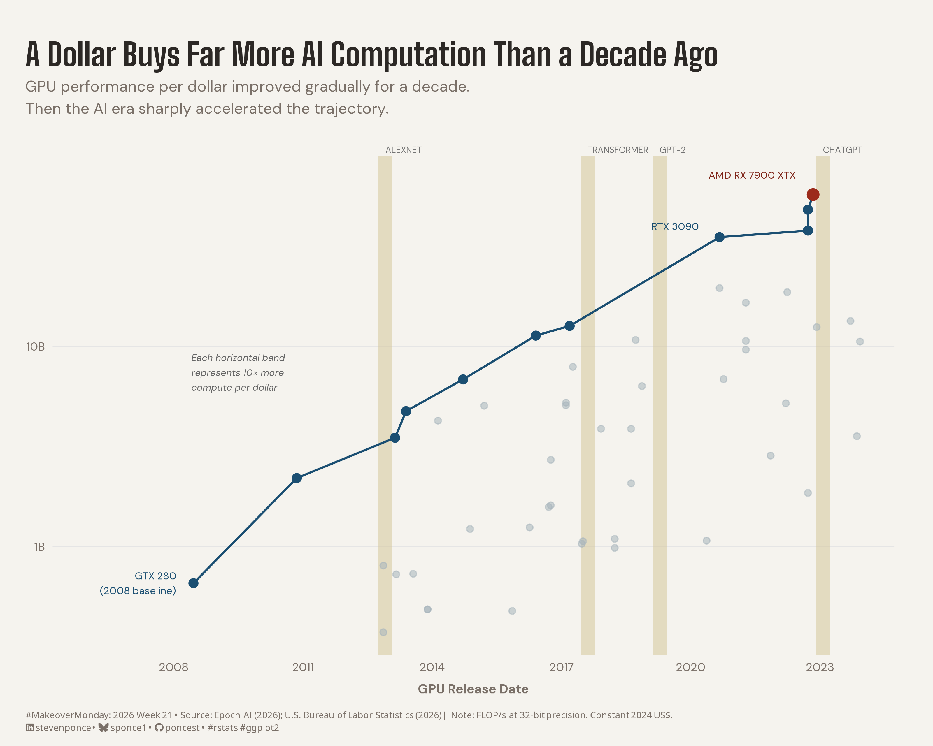
This chart shows how GPU computational performance per dollar (FLOP/s per dollar, constant 2024 US$) rose roughly 100-fold from 2008 to 2023, with the steepest acceleration coinciding with major AI milestones. A rolling frontier line identifies the best available price-performance GPU at each point in time, plotted on a log scale against a muted cloud of all 51 GPUs. Built in R using ggplot2, ggtext, and showtext.

Original

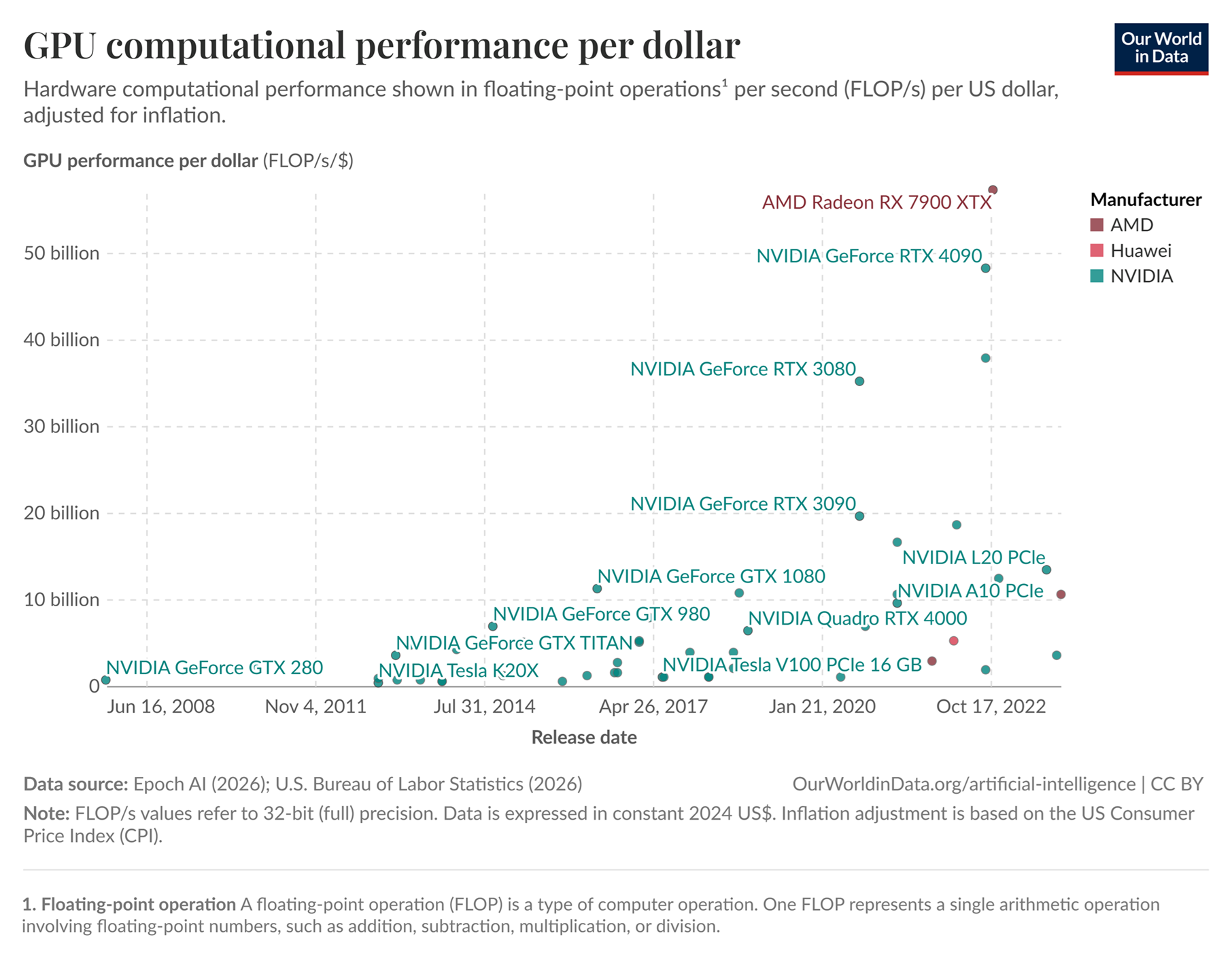
The original visualization comes from GPU computational performance per dollar

Original visualization

Makeover

Figure 1: A log-scale scatter plot titled “A Dollar Buys Far More AI Computation Than a Decade Ago” showing GPU computational performance per dollar (FLOP/s per dollar, constant 2024 US$) from 2008 to 2023. A navy frontier line connects the best available price-performance GPU at each point in time, rising from roughly 500 million FLOP/s per dollar for the NVIDIA GeForce GTX 280 in 2008 to over 50 billion for the AMD Radeon RX 7900 XTX in 2022 — a roughly 100-fold increase. The steepest acceleration occurs after 2017. Four parchment-colored vertical bands mark AI milestones: AlexNet (2012), Transformer (2017), GPT-2 (2019), and ChatGPT (2022). A muted gray cloud of all 51 GPUs provides context. Each horizontal band represents 10× more compute per dollar. Data from Epoch AI (2026) and U.S. Bureau of Labor Statistics (2026).

Steps to Create this Graphic

1. Load Packages & Setup

```{r}
#| label: load
#| warning: false
#| message: false      
#| results: "hide"     

## 1. LOAD PACKAGES & SETUP ----
suppressPackageStartupMessages({
  if (!require("pacman")) install.packages("pacman")
  pacman::p_load(
    tidyverse, ggtext, showtext, scales, 
  glue, janitor
)
})

### |- figure size ----
camcorder::gg_record(
  dir    = here::here("temp_plots"),
  device = "png",
  width  = 10,
  height = 8,
  units  = "in",
  dpi    = 320
)

# Source utility functions
suppressMessages(source(here::here("R/utils/fonts.R")))
source(here::here("R/utils/social_icons.R"))
source(here::here("R/utils/image_utils.R"))
source(here::here("R/themes/base_theme.R"))
```

2. Read in the Data

```{r}
#| label: read
#| include: true
#| eval: true
#| warning: false
#| 

df_raw <- read_csv(
  here::here("data/MakeoverMonday/2026/GPU performance per dollar.csv")) |>
  clean_names()
```

3. Examine the Data

```{r}
#| label: examine
#| include: true
#| eval: true
#| results: 'hide'
#| warning: false

glimpse(df_raw)
skimr::skim_without_charts(df_raw)
```

4. Tidy Data

```{r}
#| label: tidy
#| warning: false

### |-  parse and rename ----
df <- df_raw |>
  rename(
    gpu_name = entity,
    release_date = day,
    flops_per_dollar = gpu_performance_per_dollar
  ) |>
  arrange(release_date)

### |-  frontier: rolling maximum FLOP/s/$ over time ----
# Frontier = best available price-performance at each release date
# with_ties = FALSE prevents non-deterministic multi-row returns

df_frontier <- df |>
  arrange(release_date) |>
  mutate(
    frontier_max = cummax(flops_per_dollar),
    on_frontier = flops_per_dollar == frontier_max
  ) |>
  filter(on_frontier)

### |-  pre-extract label coordinates from df ----
gtx280_x  <- df |> filter(gpu_name == "NVIDIA GeForce GTX 280")  |> pull(release_date)
gtx280_y <- df |> filter(gpu_name == "NVIDIA GeForce GTX 280")  |> pull(flops_per_dollar)
rtx3090_x <- df |> filter(gpu_name == "NVIDIA GeForce RTX 3090") |> pull(release_date)
rtx3090_y <- df |> filter(gpu_name == "NVIDIA GeForce RTX 3090") |> pull(flops_per_dollar)
amd_x <- df |> filter(gpu_name == "AMD Radeon RX 7900 XTX")  |> pull(release_date)
amd_y <- df |> filter(gpu_name == "AMD Radeon RX 7900 XTX")  |> pull(flops_per_dollar)

### |-  AMD peak point (drawn separately with accent color) ----
df_amd_peak <- df |> filter(gpu_name == "AMD Radeon RX 7900 XTX")

### |-  AI milestone bands ----

# Four milestones
# for a societal acceleration story where ChatGPT is the public inflection)
# Band width = 120 days
milestones <- tibble(
  label = c("ALEXNET", "TRANSFORMER", "GPT-2", "CHATGPT"),
  date = as.Date(c("2012-09-30", "2017-06-12", "2019-02-14", "2022-11-30")),
  date_end = as.Date(c("2012-09-30", "2017-06-12", "2019-02-14", "2022-11-30")) + 120
)
```

5. Visualization Parameters

```{r}
#| label: params
#| include: true
#| warning: false

### |-  plot aesthetics ----
clrs <- get_theme_colors(
  palette = list(
    col_cloud = "#A8B4BC",
    col_frontier = "#1B4F72",
    col_peak = "#9C2B1B",
    col_peak_label = "#7F2418",
    col_milestone = "#D6C79A",
    col_label = "#1B4F72"
  )
)

# Unpack  — avoids $palette$ repetition in plot code
col_cloud <- clrs$palette$col_cloud
col_frontier <- clrs$palette$col_frontier
col_peak <- clrs$palette$col_peak
col_peak_label <- clrs$palette$col_peak_label
col_milestone <- clrs$palette$col_milestone
col_label <- clrs$palette$col_label

### |-  titles and caption ----
title_text <- str_glue("A Dollar Buys Far More AI Computation Than a Decade Ago")

subtitle_text <- str_glue(
  "GPU performance per dollar improved gradually for a decade.\n",
  "Then the AI era sharply accelerated the trajectory."
)

caption_text <- create_mm_caption(
  mm_year = 2026,
  mm_week = 21,
  source_text = "Epoch AI (2026); U.S. Bureau of Labor Statistics (2026) |
  Note: FLOP/s at 32-bit precision. Constant 2024 US$."
)

### |-  fonts ----
setup_fonts()
fonts <- get_font_families()

### |-  plot theme ----
base_theme <- create_base_theme(clrs)

weekly_theme <- extend_weekly_theme(
  base_theme,
  theme(
    # Title / subtitle
    plot.title.position = "plot",
    plot.title = element_text(size = 24, face = "bold", family = fonts$title_1, 
                              color = clrs$title, margin = margin(b = 6)),
    plot.subtitle = element_text(size = 12, family = fonts$subtitle, lineheight = 1.2, 
                                 color = clrs$subtitle, margin = margin(b = 30)),

    # Caption
    plot.caption = element_markdown(
      size = 7, hjust = 0, lineheight = 1.4, family = fonts$caption,
      margin = margin(t = 12), color = clrs$caption
    ),

    # Axes
    axis.title.x = element_text(size = 10, margin = margin(t = 8)),
    axis.title.y = element_blank(),
    axis.text.x = element_text(size = 9),
    axis.text.y = element_text(size = 9),
    axis.ticks = element_blank(),

    # Grid — y-lines only
    panel.grid.major.y = element_line(color = "gray90", linewidth = 0.3),
    panel.grid.major.x = element_blank(),
    panel.grid.minor = element_blank(),

    # Top margin 
    plot.margin = margin(t = 32, r = 30, b = 10, l = 20)
  )
)

theme_set(weekly_theme)
```

6. Plot

```{r}
#| label: plot
#| warning: false

### |-  y-axis label helper ----
flops_labels <- function(x) {
  case_when(
    x >= 1e9 ~ paste0(round(x / 1e9), "B"),
    x >= 1e6 ~ paste0(round(x / 1e6), "M"),
    TRUE ~ scales::comma(x)
  )
}

### |-  main plot ----
p <- ggplot() +
  # Geoms
  geom_rect(
    data = milestones,
    aes(xmin = date, xmax = date_end),
    ymin = -Inf,
    ymax = Inf,
    fill = col_milestone,
    alpha = 0.55,
    inherit.aes = FALSE
  ) +
  geom_text(
    data = milestones,
    aes(x = date + 60, y = Inf, label = label),
    vjust = -0.5,
    hjust = 0,
    size = 2.4,
    color = "gray45",
    fontface = "plain",
    inherit.aes = FALSE
  ) +
  geom_point(
    data = df,
    aes(x = release_date, y = flops_per_dollar),
    color = col_cloud,
    size = 2,
    alpha = 0.55
  ) +
  geom_line(
    data = df_frontier,
    aes(x = release_date, y = flops_per_dollar),
    color = col_frontier,
    linewidth = 0.78,
    lineend = "round"
  ) +
  geom_point(
    data = df_frontier,
    aes(x = release_date, y = flops_per_dollar),
    color = col_frontier,
    size = 2.8
  ) +
  geom_point(
    data = df_amd_peak,
    aes(x = release_date, y = flops_per_dollar),
    color = col_peak,
    size = 3.8
  ) +
  # Annotate
  annotate(
    "text",
    x = gtx280_x - 150,
    y = gtx280_y,
    label = "GTX 280\n(2008 baseline)",
    hjust = 1,
    vjust = 0.5,
    size = 2.8,
    color = col_label,
    lineheight = 1.2
  ) +
  annotate(
    "text",
    x = rtx3090_x - 180,
    y = rtx3090_y * 1.95,
    label = "RTX 3090",
    hjust = 1,
    vjust = 0,
    size = 2.8,
    color = col_label,
    lineheight = 1.2
  ) +
  annotate(
    "text",
    x = amd_x - 150,
    y = amd_y * 1.2,
    label = "AMD RX 7900 XTX",
    hjust = 1,
    vjust = 0,
    size = 2.8,
    color = col_peak_label,
    lineheight = 1.2
  ) +
  annotate(
    "text",
    x = as.Date("2008-06-01"),
    y = 6e9,
    label = "Each horizontal band\nrepresents 10× more\ncompute per dollar",
    hjust = 0,
    vjust = 0,
    size = 2.6,
    color = "gray40",
    lineheight = 1.3,
    fontface = "italic"
  ) +
  # Scales
  scale_y_log10(
    labels = flops_labels,
    breaks = c(1e8, 1e9, 1e10, 1e11)
  ) +
  scale_x_date(
    date_breaks = "3 years",
    date_labels = "%Y",
    expand = expansion(mult = c(0.18, 0.05))
  ) +
  coord_cartesian(clip = "off") +
  # Labs
  labs(
    title = title_text,
    subtitle = subtitle_text,
    caption = caption_text,
    x = "GPU Release Date",
    y = NULL
  )
```

7. Save

```{r}
#| label: save
#| warning: false

### |-  plot image ----  
save_plot(
  plot = p, 
  type = "makeovermonday", 
  year = current_year,
  week = current_week,
  width = 10, 
  height = 8
  )
```

8. Session Info

TipExpand for Session Info

R version 4.5.3 (2026-03-11 ucrt)
Platform: x86_64-w64-mingw32/x64
Running under: Windows 11 x64 (build 26100)

Matrix products: default
  LAPACK version 3.12.1

locale:
[1] LC_COLLATE=English_United States.utf8 
[2] LC_CTYPE=English_United States.utf8   
[3] LC_MONETARY=English_United States.utf8
[4] LC_NUMERIC=C                          
[5] LC_TIME=English_United States.utf8    

time zone: America/New_York
tzcode source: internal

attached base packages:
[1] stats     graphics  grDevices utils     datasets  methods   base     

other attached packages:
 [1] here_1.0.2      janitor_2.2.1   glue_1.8.0      scales_1.4.0   
 [5] showtext_0.9-8  showtextdb_3.0  sysfonts_0.8.9  ggtext_0.1.2   
 [9] lubridate_1.9.5 forcats_1.0.1   stringr_1.6.0   dplyr_1.2.1    
[13] purrr_1.2.2     readr_2.2.0     tidyr_1.3.2     tibble_3.3.1   
[17] ggplot2_4.0.3   tidyverse_2.0.0 pacman_0.5.1   

loaded via a namespace (and not attached):
 [1] gtable_0.3.6       xfun_0.57          htmlwidgets_1.6.4  tzdb_0.5.0        
 [5] vctrs_0.7.3        tools_4.5.3        generics_0.1.4     curl_7.0.0        
 [9] parallel_4.5.3     gifski_1.32.0-2    pkgconfig_2.0.3    skimr_2.2.2       
[13] RColorBrewer_1.1-3 S7_0.2.1           lifecycle_1.0.5    compiler_4.5.3    
[17] farver_2.1.2       textshaping_1.0.5  repr_1.1.7         codetools_0.2-20  
[21] snakecase_0.11.1   litedown_0.9       htmltools_0.5.9    yaml_2.3.12       
[25] pillar_1.11.1      crayon_1.5.3       camcorder_0.1.0    magick_2.9.1      
[29] commonmark_2.0.0   tidyselect_1.2.1   digest_0.6.39      stringi_1.8.7     
[33] rsvg_2.7.0         rprojroot_2.1.1    fastmap_1.2.0      grid_4.5.3        
[37] cli_3.6.6          magrittr_2.0.5     base64enc_0.1-6    withr_3.0.2       
[41] bit64_4.6.0-1      timechange_0.4.0   rmarkdown_2.31     bit_4.6.0         
[45] otel_0.2.0         ragg_1.5.2         hms_1.1.4          evaluate_1.0.5    
[49] knitr_1.51         markdown_2.0       rlang_1.2.0        gridtext_0.1.6    
[53] Rcpp_1.1.1         xml2_1.5.2         svglite_2.2.2      rstudioapi_0.18.0 
[57] vroom_1.7.1        jsonlite_2.0.0     R6_2.6.1           systemfonts_1.3.2 

9. GitHub Repository

TipExpand for GitHub Repo

The complete code for this analysis is available in mm_2026_21.qmd.

For the full repository, click here.

10. References

TipExpand for References

Primary Data (Makeover Monday): 1. Makeover Monday 2026 Week 21: GPU Computational Performance per Dollar 2. Original Chart: Our World in Data — GPU Price-Performance - Source: Epoch AI (2026); U.S. Bureau of Labor Statistics (2026) - Coverage: 51 GPUs from June 2008 to December 2023 across three manufacturers (AMD, Huawei, NVIDIA)

Source Data: 3. Epoch AI — GPU Performance per Dollar - Coverage: GPU computational performance measured in floating-point operations per second (FLOP/s) per US dollar - Unit: FLOP/s per dollar; 32-bit (full) precision; inflation-adjusted to constant 2024 US$ using US CPI 4. MakeoverMonday 2026 W21 — data.world - CSV file: GPU performance per dollar.csv; 51 rows × 4 columns (entity, day, gpu_performance_per_dollar, manufacturer)

AI Milestone Reference Dates: 5. AlexNet — Krizhevsky, A., Sutskever, I., & Hinton, G. E. (2012). ImageNet classification with deep convolutional neural networks. NeurIPS. September 30, 2012. 6. Transformer — Vaswani, A., et al. (2017). Attention is all you need. NeurIPS. June 12, 2017. 7. GPT-2 — Radford, A., et al. (2019). Language models are unsupervised multitask learners. OpenAI. February 14, 2019. 8. ChatGPT — OpenAI. (2022). ChatGPT: Optimizing language models for dialogue. November 30, 2022. openai.com/blog/chatgpt

Note: The frontier line represents the rolling maximum FLOP/s per dollar at each GPU release date — the best available price-performance at any given point in time (cummax(flops_per_dollar)). GPUs below the frontier at their release date appear in the muted gray cloud. Milestone bands are 120-day windows centered on each publication date, included to show temporal proximity between AI capability breakthroughs and the GPU efficiency frontier — no causal relationship is asserted. Inflation adjustment uses the US Consumer Price Index (CPI) as reported by the U.S. Bureau of Labor Statistics.

11. Custom Functions Documentation

Note📦 Custom Helper Functions

This analysis uses custom functions from my personal module library for efficiency and consistency across projects.

Functions Used:

• fonts.R: setup_fonts(), get_font_families() - Font management with showtext
• social_icons.R: create_social_caption() - Generates formatted social media captions
• image_utils.R: save_plot() - Consistent plot saving with naming conventions
• base_theme.R: create_base_theme(), extend_weekly_theme(), get_theme_colors() - Custom ggplot2 themes

Why custom functions?
These utilities standardize theming, fonts, and output across all my data visualizations. The core analysis (data tidying and visualization logic) uses only standard tidyverse packages.

Source Code:
View all custom functions → GitHub: R/utils