• Steven Ponce
  • About
  • Data Visualizations
  • Projects
  • Resume
  • Email

On this page

  • Original
  • Makeover
  • Steps to Create this Graphic
    • 1. Load Packages & Setup
    • 2. Read in the Data
    • 3. Examine the Data
    • 4. Tidy Data
    • 5. Visualization Parameters
    • 6. Plot
    • 7. Save
    • 8. Session Info
    • 9. GitHub Repository
    • 10. References
    • 11. Custom Functions Documentation

Central Manhattan Recorded the Highest Share of Stationary Squirrels

  • Show All Code
  • Hide All Code

  • View Source

Four Central Manhattan parks ranked among the city’s highest, but the pattern wasn’t universal—or exclusive to the area

MakeoverMonday
Data Visualization
R Programming
2026
A two-panel chart comparing squirrel behavior across NYC’s 2020 multi-park census: stacked bars show Central Manhattan squirrels recorded stationary 54% of the time versus 33–34% elsewhere, while a park-level ranking tests whether that pattern holds within and beyond Central Manhattan. Built in R with ggplot2, patchwork, and ggview.
Author

Steven Ponce

Published

July 27, 2026

Original

No ‘original chart’ was provided.

Makeover

Figure 1: Two-panel chart titled “Central Manhattan Recorded the Highest Share of Stationary Squirrels.” Top panel: stacked bars show behavioral composition by NYC census area from the 2020 Squirrel Census multi-park count — Central Manhattan squirrels were recorded stationary (foraging or eating) 54% of the time, versus 33–34% in Lower Manhattan, Brooklyn, and Upper Manhattan. Bottom panel: a dot plot ranks all 20 sampled parks by stationary share. Four Central Manhattan parks cluster near the top, but St. Nicholas Park (Upper Manhattan) sits within that high-stationary cluster, while John V. Lindsay East River Park (Central Manhattan) falls below the citywide median — showing that the area-level pattern was neither universal within Central Manhattan nor exclusive to it.

Steps to Create this Graphic

1. Load Packages & Setup

Show code
```{r}
#| label: load
#| warning: false
#| message: false      
#| results: "hide"     

## 1. LOAD PACKAGES & SETUP ----
suppressPackageStartupMessages({
  if (!require("pacman")) install.packages("pacman")
  pacman::p_load(
    tidyverse, ggtext, showtext, scales, glue, 
  janitor, ggview, patchwork
)
})

# Source utility functions
suppressMessages(source(here::here("R/utils/fonts.R")))
source(here::here("R/utils/social_icons.R"))
source(here::here("R/themes/base_theme.R"))
```

2. Read in the Data

Show code
```{r}
#| label: read
#| include: true
#| eval: true
#| warning: false
#| 

df_raw <- read_csv(
  here::here("data/MakeoverMonday/2026/squirrel-data.csv"))  |>
  clean_names()
```

3. Examine the Data

Show code
```{r}
#| label: examine
#| include: true
#| eval: true
#| results: 'hide'
#| warning: false

glimpse(df_raw)
skimr::skim_without_charts(df_raw)
```

4. Tidy Data

Show code
```{r}
#| label: tidy
#| warning: false

### |- classify behavior state ----
# `activities` is a comma-separated, multi-value field.
stationary_acts <- c("Foraging", "Eating")
movement_acts <- c("Running", "Chasing", "Climbing")

df_behavior <- df_raw |>
  select(squirrel_id, area_name, park_name, activities) |>
  filter(!is.na(activities)) |>
  separate_longer_delim(activities, delim = ", ") |>
  mutate(activities = str_trim(activities)) |>
  summarize(
    has_stationary = any(activities %in% stationary_acts),
    has_movement = any(activities %in% movement_acts),
    .by = c(squirrel_id, area_name, park_name)
  ) |>
  mutate(
    behavior_state = case_when(
      has_stationary & has_movement ~ "Both",
      has_stationary & !has_movement ~ "Stationary",
      !has_stationary & has_movement ~ "Movement",
      TRUE ~ "Other"
    ),
    area_name = str_to_title(area_name)
  )

### |- area-level composition ----
df_area <- df_behavior |>
  count(area_name, behavior_state) |>
  mutate(pct = n / sum(n) * 100, .by = area_name) |>
  mutate(
    behavior_state = factor(
      behavior_state,
      levels = c("Stationary", "Both", "Other", "Movement")
    )
  )

# order areas by stationary share, descending
area_order <- df_behavior |>
  summarize(pct_stationary = mean(behavior_state == "Stationary") * 100, .by = area_name) |>
  arrange(desc(pct_stationary)) |>
  pull(area_name)

df_area <- df_area |>
  mutate(area_name = factor(area_name, levels = rev(area_order)))

### |- park-level summary ----
df_park <- df_behavior |>
  summarize(
    n = n(),
    pct_stationary = mean(behavior_state == "Stationary") * 100,
    .by = c(area_name, park_name)
  ) |>
  mutate(
    is_central_manhattan = area_name == "Central Manhattan",
    flag_small_n = n < 10,
    park_name_label = if_else(
      park_name == "Washington Square Park",
      glue("{park_name} \u2020"),
      park_name
    ),
    park_label = fct_reorder(park_name_label, pct_stationary)
  )

### |- citywide reference line ----
citywide_pct_stationary <- mean(df_behavior$behavior_state == "Stationary") * 100

### |- pre-extracted annotation coordinates ----
st_nicholas_x <- df_park |> filter(park_name == "St. Nicholas Park") |>
  pull(pct_stationary)

st_nicholas_label <- df_park |> filter(park_name == "St. Nicholas Park") |>
  pull(park_label) |> as.character()

lindsay_x <- df_park |>
  filter(park_name == "John V. Lindsay East River Park") |> pull(pct_stationary)

lindsay_label <- df_park |>
  filter(park_name == "John V. Lindsay East River Park") |> pull(park_label) |>
  as.character()
```

5. Visualization Parameters

Show code
```{r}
#| label: params
#| include: true
#| warning: false

### |- plot aesthetics ----
theme_colors <- get_theme_colors(
  palette = list(
    stationary   = "#8C5A3C",
    movement     = "#B8B8B8",
    both         = "#D8C3AE",
    other        = "#E8E8E8",
    accent       = "#2C5F8D",
    neutral_dark = "#3A3A3A"
  )
)
clrs <- theme_colors$palette

### |- titles and caption ----
title_text <- str_glue("Central Manhattan Recorded the Highest Share of Stationary Squirrels")

subtitle_text <- str_glue(
  "Four Central Manhattan parks ranked among the city's highest, but the<br>",
  "pattern wasn't universal\u2014or exclusive to the area"
)

caption_text <- create_mm_caption(
  mm_year = 2026,
  mm_week = 30,
  source_text = "The Squirrel Census, 2020 NYC Open Data Week Multi-Park Sample Count<br>Activities grouped as Stationary (Foraging, Eating) or Movement (Running, Chasing, Climbing). One Upper Manhattan park ranked with the Central Manhattan cluster, while one Central Manhattan park fell below the city median."
)

### |- fonts ----
setup_fonts()
fonts <- get_font_families()

### |- plot theme ----
base_theme <- create_base_theme(theme_colors)

weekly_theme <- extend_weekly_theme(
  base_theme,
  theme(
    plot.title = element_text(size = 22, face = "bold", margin = margin(b = 4), family = fonts$title_1, lineheight = 1.15),
    plot.subtitle = element_markdown(size = 13, color = clrs$neutral_dark, margin = margin(b = 12), family = fonts$subtitle, lineheight = 1.15),
    plot.caption = element_textbox_simple(size = 7, color = "gray50", margin = margin(t = 10), family = fonts$caption),
    legend.title = element_text(size = 10, face = "plain"),
    legend.text = element_text(size = 9),
    legend.position = "bottom",
    panel.grid.major.y = element_blank(),
    panel.grid.major.x = element_line(color = "gray90", linewidth = 0.3),
    panel.grid.minor = element_blank(),
    axis.ticks = element_blank()
  )
)

theme_set(weekly_theme)
```

6. Plot

Show code
```{r}
#| label: plot
#| warning: false

### |- panel 1: area-level composition ----
p_area <- ggplot(df_area, aes(x = pct, y = area_name, fill = behavior_state)) +
  geom_col(width = 0.65) +
  geom_text(
    data = df_area |> filter(behavior_state == "Stationary"),
    aes(x = 100 - pct / 2, label = paste0(round(pct), "% stationary")),
    color = "white", fontface = "bold", size = 4
  ) +
  scale_fill_manual(
    name = "Behavioral state",
    values = c(
      "Stationary" = clrs$stationary,
      "Both"       = clrs$both,
      "Other"      = clrs$other,
      "Movement"   = clrs$movement
    )
  ) +
  guides(fill = guide_legend(reverse = TRUE)) +
  scale_x_continuous(expand = c(0, 0)) +
  labs(subtitle = "Behavioral composition by area", x = NULL, y = NULL) +
  theme(
    axis.text.x = element_blank(),
    plot.subtitle = element_markdown(size = 10, face = "bold", color = "gray30", margin = margin(b = 8))
  )

### |- panel 2: park-level ranking ----
p_park <- ggplot(df_park, aes(x = pct_stationary, y = park_label)) +
  geom_vline(xintercept = citywide_pct_stationary, color = "gray80", linewidth = 0.4) +
  geom_segment(aes(x = 0, xend = pct_stationary, yend = park_label),
    color = "gray85", linewidth = 0.4
  ) +
  geom_point(aes(color = is_central_manhattan, shape = flag_small_n), size = 2.5) +
  annotate(
    "text",
    x = st_nicholas_x + 4, y = st_nicholas_label,
    label = "Upper Manhattan park\ninside the cluster",
    hjust = 0, size = 3, color = clrs$accent, lineheight = 0.9
  ) +
  annotate(
    "text",
    x = lindsay_x - 4, y = lindsay_label,
    label = "Central Manhattan park\nbelow the median",
    hjust = 1, size = 3, color = clrs$accent, lineheight = 0.9
  ) +
  scale_color_manual(
    values = c("TRUE" = clrs$stationary, "FALSE" = "gray70"),
    guide = "none"
  ) +
  scale_shape_manual(values = c("FALSE" = 16, "TRUE" = 1), guide = "none") +
  scale_x_continuous(limits = c(0, 100), expand = c(0, 0)) +
  labs(
    subtitle = "Stationary share by park",
    x = "Percent of squirrels recorded stationary",
    y = NULL,
    caption = "Hollow points denote fewer than 10 usable activity records. \u2020 Washington Square Park had substantial missing activity data."
  ) +
  theme(
    axis.text.y = element_text(size = 8),
    plot.subtitle = element_markdown(size = 10, face = "bold", color = "gray30", margin = margin(b = 8)),
    plot.caption = element_textbox_simple(size = 7, color = "gray50")
  )

### |- combine with patchwork ----
combined_plot <- p_area / p_park +
  plot_layout(heights = c(1, 2.5), guides = "collect") &
  theme(
    legend.position = "bottom",
    legend.box.spacing = unit(2, "pt")
  )

combined_plot <- combined_plot +
  plot_annotation(
    title = title_text,
    subtitle = subtitle_text,
    caption = caption_text,
    theme = weekly_theme
  ) +
  canvas(width = 10, height = 9.5, units = "in")
```

7. Save

Show code
```{r}
#| label: save
#| warning: false

### |- save ----
main_path  <- here::here("data_visualizations", "MakeoverMonday", "2026", "mm_2026_30.png")
thumb_path <- here::here("data_visualizations", "MakeoverMonday", "2026", "thumbnails", "mm_2026_30.png")

# Full-size version, for the QMD figure
save_ggplot(
  plot = combined_plot,
  file = main_path,
  width = 10,
  height = 9.5,
  units = "in",
  dpi = 320,
  create.dir = TRUE
)

# Reduced-size thumbnail, for the YAML `image:` field
fs::dir_create(dirname(thumb_path))
magick::image_read(main_path) |>
  magick::image_resize("400") |>
  magick::image_write(thumb_path)
```

8. Session Info

TipExpand for Session Info
R version 4.6.1 (2026-06-24)
Platform: aarch64-apple-darwin23
Running under: macOS Tahoe 26.5.2

Matrix products: default
BLAS:   /Library/Frameworks/R.framework/Versions/4.6/Resources/lib/libRblas.0.dylib 
LAPACK: /Library/Frameworks/R.framework/Versions/4.6/Resources/lib/libRlapack.dylib;  LAPACK version 3.12.1

locale:
[1] en_US.UTF-8/en_US.UTF-8/en_US.UTF-8/C/en_US.UTF-8/en_US.UTF-8

time zone: America/New_York
tzcode source: internal

attached base packages:
[1] stats     graphics  grDevices utils     datasets  methods   base     

other attached packages:
 [1] here_1.0.2      patchwork_1.3.2 ggview_0.2.2    janitor_2.2.1  
 [5] glue_1.8.1      scales_1.4.0    showtext_0.9-8  showtextdb_3.0 
 [9] sysfonts_0.8.9  ggtext_0.1.2    lubridate_1.9.5 forcats_1.0.1  
[13] stringr_1.6.0   dplyr_1.2.1     purrr_1.2.2     readr_2.2.0    
[17] tidyr_1.3.2     tibble_3.3.1    ggplot2_4.0.3   tidyverse_2.0.0
[21] pacman_0.5.1   

loaded via a namespace (and not attached):
 [1] gtable_0.3.6       xfun_0.60          htmlwidgets_1.6.4  tzdb_0.5.0        
 [5] vctrs_0.7.3        tools_4.6.1        generics_0.1.4     curl_7.1.0        
 [9] parallel_4.6.1     pkgconfig_2.0.3    RColorBrewer_1.1-3 skimr_2.2.2       
[13] S7_0.2.2           lifecycle_1.0.5    compiler_4.6.1     farver_2.1.2      
[17] textshaping_1.0.5  repr_1.1.7         codetools_0.2-20   snakecase_0.11.1  
[21] litedown_0.10      htmltools_0.5.9    yaml_2.3.12        pillar_1.11.1     
[25] crayon_1.5.3       magick_2.9.1       commonmark_2.0.0   tidyselect_1.2.1  
[29] digest_0.6.39      stringi_1.8.7      labeling_0.4.3     rprojroot_2.1.1   
[33] fastmap_1.2.0      grid_4.6.1         cli_3.6.6          magrittr_2.0.5    
[37] base64enc_0.1-6    withr_3.0.3        bit64_4.8.2        timechange_0.4.0  
[41] rmarkdown_2.31     bit_4.6.0          otel_0.2.0         ragg_1.5.2        
[45] hms_1.1.4          evaluate_1.0.5     knitr_1.51         markdown_2.0      
[49] rlang_1.3.0        gridtext_0.1.6     Rcpp_1.1.2         xml2_1.6.0        
[53] rstudioapi_0.19.0  vroom_1.7.1        jsonlite_2.0.0     R6_2.6.1          
[57] fs_2.1.0           systemfonts_1.3.2 

9. GitHub Repository

TipExpand for GitHub Repo

The complete code for this analysis is available in mm_2026_30.qmd.

For the full repository, click here.

10. References

TipExpand for References

Primary Data (Makeover Monday):

  1. Makeover Monday 2026 Week 30: Squirrel Census 2020
    • CSV: 433 rows × 16 columns. Each record represents a single squirrel sighting from a 2020 NYC Open Data Week multi-park count, with fields covering location (area, park, coordinates), fur color, activities, human interaction, and free-text observation notes.
    • No original visualization was published alongside this dataset, so this makeover was built directly from the raw data rather than as a redesign of an existing chart. Phase 0 exploratory analysis tested and discarded several candidate stories (fur color composition, height/vertical ecology, activity co-occurrence networks) before a behavioral-state finding — squirrels observed stationary vs. in movement — survived repeated falsification attempts.

Source Data:

  1. The Squirrel Census — Data
    • The 2020 NYC Open Data Week multi-park sample count, compiled by The Squirrel Census as a smaller-scale companion effort to their 2018 Central Park census, covering 20 parks across four NYC census areas (Central Manhattan, Upper Manhattan, Lower Manhattan, Brooklyn).
    • This visualization uses the area_name, park_name, and activities fields. Fur color, human interaction, and free-text note fields were reviewed during exploratory analysis but are not shown in the published chart, once the color-composition story was ruled out as a single-park artifact (see Methodological Notes).

Methodological Notes:

  1. Squirrel-level activity records were classified into a four-category behavioral state, replacing the source’s five-plus free-text activity field:
    • Stationary: Foraging, Eating
    • Movement: Running, Chasing, Climbing
    • Both: record contains at least one activity from each group
    • Other: record has an activity, but none map to Stationary or Movement (e.g., “Sitting,” “Defending tree, shouting”)
    • This collapse was tested for robustness under all three defensible treatments of the ambiguous “Climbing” case (Movement / Stationary / excluded); the area-level result held under all three. “Climbing → Movement” was locked as final since a squirrel changing position is the clearest one-sentence justification.
  2. The area-level finding (Central Manhattan highest stationary share) was deliberately re-tested at the park level after an initial version overstated it. Standardized residuals showed the original color-composition claim was driven by a single park (McCarren Park, Brooklyn) rather than an area-wide pattern, and was dropped; the behavioral-state finding held under the same scrutiny, including a gray-squirrels-only subset that removes color as a confound.
  3. park-data.csv, which would contain park-level characteristics (size, canopy cover, visitor volume) potentially explaining the behavioral pattern, was not released with this dataset and was not available from The Squirrel Census’s public data page. The finding is therefore reported as an observed association (“squirrels observed… were more likely to be recorded…”) rather than an explained cause, and that boundary is stated in the chart’s caption rather than implied by the title.
  4. Three parks (Columbus Park, Teardrop Park, Seward Park) had fewer than 10 usable activity records and are flagged with hollow point markers in the park-level panel rather than excluded, since their direction is still informative even at low precision. Washington Square Park had substantial activity-field missingness (70.6%) unrelated to the other five Central Manhattan parks in the sample and is flagged separately in the chart caption.

11. Custom Functions Documentation

Note📦 Custom Helper Functions

This analysis uses custom functions from my personal module library for efficiency and consistency across projects.

Functions Used:

  • fonts.R: setup_fonts(), get_font_families() - Font management with showtext
  • social_icons.R: create_social_caption() - Generates formatted social media captions
  • image_utils.R: save_plot() - Consistent plot saving with naming conventions
  • base_theme.R: create_base_theme(), extend_weekly_theme(), get_theme_colors() - Custom ggplot2 themes

Why custom functions?
These utilities standardize theming, fonts, and output across all my data visualizations. The core analysis (data tidying and visualization logic) uses only standard tidyverse packages.

Source Code:
View all custom functions → GitHub: R/utils

Back to top

Citation

BibTeX citation:
@online{ponce2026,
  author = {Ponce, Steven},
  title = {Central {Manhattan} {Recorded} the {Highest} {Share} of
    {Stationary} {Squirrels}},
  date = {2026-07-27},
  url = {https://stevenponce.netlify.app/data_visualizations/MakeoverMonday/2026/mm_2026_30.html},
  langid = {en}
}
For attribution, please cite this work as:
Ponce, Steven. 2026. “Central Manhattan Recorded the Highest Share of Stationary Squirrels.” July 27. https://stevenponce.netlify.app/data_visualizations/MakeoverMonday/2026/mm_2026_30.html.
Source Code
---
title: "Central Manhattan Recorded the Highest Share of Stationary Squirrels"
subtitle: "Four Central Manhattan parks ranked among the city's highest, but the pattern wasn't universal—or exclusive to the area"
description: "A two-panel chart comparing squirrel behavior across NYC's 2020 multi-park census: stacked bars show Central Manhattan squirrels recorded stationary 54% of the time versus 33–34% elsewhere, while a park-level ranking tests whether that pattern holds within and beyond Central Manhattan. Built in R with ggplot2, patchwork, and ggview."
date: "2026-07-27"
author:
  - name: "Steven Ponce"
    url: "https://stevenponce.netlify.app"
citation:
  url: "https://stevenponce.netlify.app/data_visualizations/MakeoverMonday/2026/mm_2026_30.html"
categories: ["MakeoverMonday", "Data Visualization", "R Programming", "2026"]
tags: [
  "makeover-monday",
  "data-visualization",
  "ggplot2",
  "stacked-bar-chart",
  "dot-plot",
  "patchwork",
  "nyc",
  "squirrel-census",
  "urban-wildlife",
  "behavioral-data",
  "annotation",
  "2026"
]
image: "thumbnails/mm_2026_30.png"
format:
  html:
    toc: true
    toc-depth: 5
    code-link: true
    code-fold: true
    code-tools: true
    code-summary: "Show code"
    self-contained: true
    theme: 
      light: [flatly, assets/styling/custom_styles.scss]
      dark: [darkly, assets/styling/custom_styles_dark.scss]
editor_options: 
  chunk_output_type: inline
execute: 
  freeze: true
  cache: true
  error: false
  message: false
  warning: false
  eval: true
---

```{r}
#| label: setup-links
#| include: false

# CENTRALIZED LINK MANAGEMENT

## Project-specific info 
current_year <- 2026
current_week <- 30
project_file <- "mm_2026_30.qmd"
project_image <- "mm_2026_30.png"

## Data Sources
data_main <- "https://makeovermonday.vercel.app/dataset/squirrel-census-2020"
data_secondary <- "https://makeovermonday.vercel.app/dataset/squirrel-census-2020"

## Repository Links  
repo_main <- "https://github.com/poncest/personal-website/"
repo_file <- paste0("https://github.com/poncest/personal-website/blob/master/data_visualizations/MakeoverMonday/", current_year, "/", project_file)

## External Resources/Images
chart_original <- "https://raw.githubusercontent.com/poncest/MakeoverMonday/refs/heads/master/2026/Week_30_original_chart.png"

## Organization/Platform Links
org_primary <- "https://www.thesquirrelcensus.com"
org_secondary <- "https://www.thesquirrelcensus.com"

# Helper function to create markdown links
create_link <- function(text, url) {
  paste0("[", text, "](", url, ")")
}

# Helper function for citation-style links
create_citation_link <- function(text, url, title = NULL) {
  if (is.null(title)) {
    paste0("[", text, "](", url, ")")
  } else {
    paste0("[", text, "](", url, ' "', title, '")')
  }
}
```

### Original

No 'original chart' was provided.

### Makeover
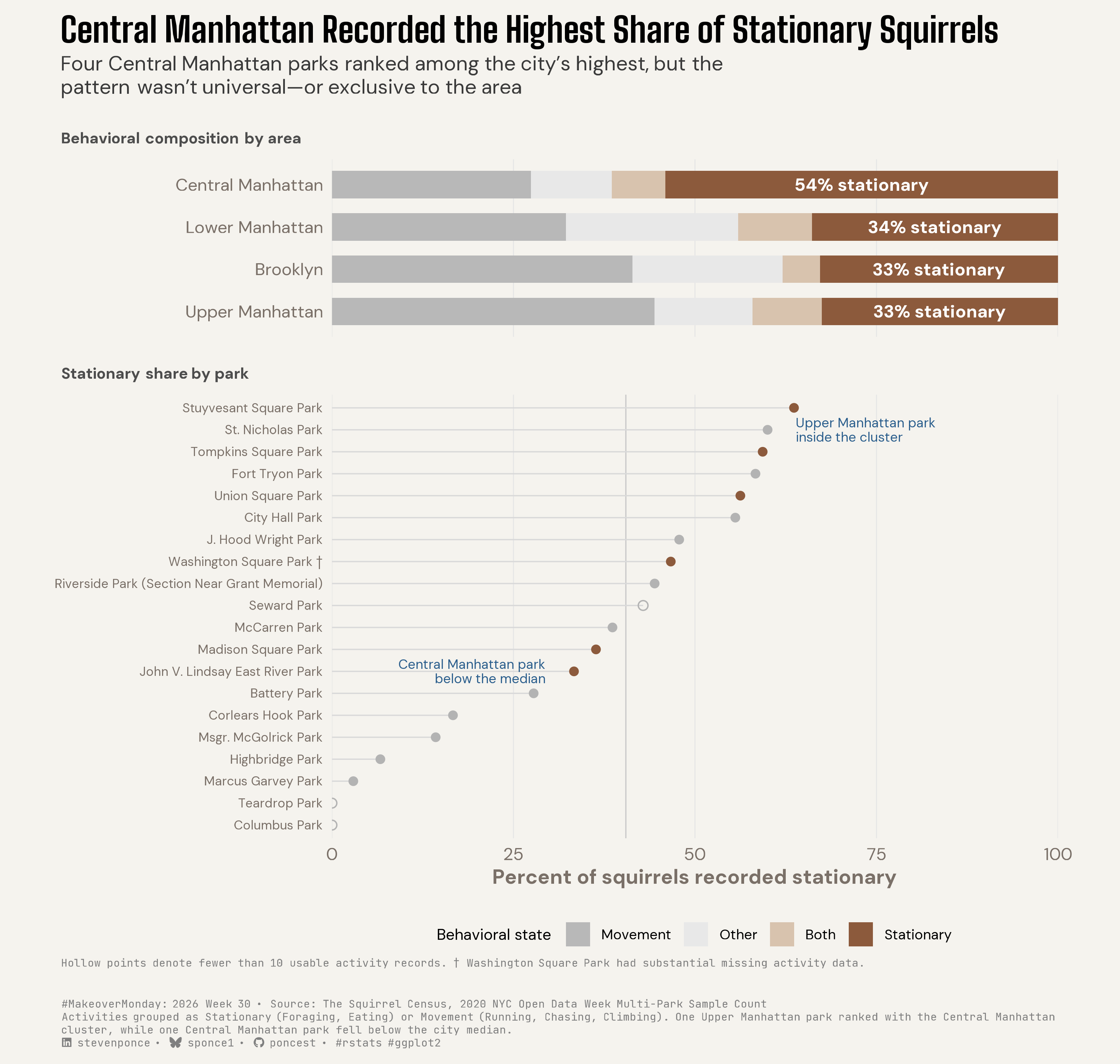
![Two-panel chart titled "Central Manhattan Recorded the Highest Share of Stationary Squirrels." Top panel: stacked bars show behavioral composition by NYC census area from the 2020 Squirrel Census multi-park count — Central Manhattan squirrels were recorded stationary (foraging or eating) 54% of the time, versus 33–34% in Lower Manhattan, Brooklyn, and Upper Manhattan. Bottom panel: a dot plot ranks all 20 sampled parks by stationary share. Four Central Manhattan parks cluster near the top, but St. Nicholas Park (Upper Manhattan) sits within that high-stationary cluster, while John V. Lindsay East River Park (Central Manhattan) falls below the citywide median — showing that the area-level pattern was neither universal within Central Manhattan nor exclusive to it.](mm_2026_30.png){#fig-1}

### [**Steps to Create this Graphic**]{.mark}

#### [1. Load Packages & Setup]{.smallcaps}

```{r}
#| label: load
#| warning: false
#| message: false      
#| results: "hide"     

## 1. LOAD PACKAGES & SETUP ----
suppressPackageStartupMessages({
  if (!require("pacman")) install.packages("pacman")
  pacman::p_load(
    tidyverse, ggtext, showtext, scales, glue, 
  janitor, ggview, patchwork
)
})

# Source utility functions
suppressMessages(source(here::here("R/utils/fonts.R")))
source(here::here("R/utils/social_icons.R"))
source(here::here("R/themes/base_theme.R"))
```

#### [2. Read in the Data]{.smallcaps}

```{r}
#| label: read
#| include: true
#| eval: true
#| warning: false
#| 

df_raw <- read_csv(
  here::here("data/MakeoverMonday/2026/squirrel-data.csv"))  |>
  clean_names()
```

#### [3. Examine the Data]{.smallcaps}

```{r}
#| label: examine
#| include: true
#| eval: true
#| results: 'hide'
#| warning: false

glimpse(df_raw)
skimr::skim_without_charts(df_raw)
```

#### [4. Tidy Data]{.smallcaps}

```{r}
#| label: tidy
#| warning: false

### |- classify behavior state ----
# `activities` is a comma-separated, multi-value field.
stationary_acts <- c("Foraging", "Eating")
movement_acts <- c("Running", "Chasing", "Climbing")

df_behavior <- df_raw |>
  select(squirrel_id, area_name, park_name, activities) |>
  filter(!is.na(activities)) |>
  separate_longer_delim(activities, delim = ", ") |>
  mutate(activities = str_trim(activities)) |>
  summarize(
    has_stationary = any(activities %in% stationary_acts),
    has_movement = any(activities %in% movement_acts),
    .by = c(squirrel_id, area_name, park_name)
  ) |>
  mutate(
    behavior_state = case_when(
      has_stationary & has_movement ~ "Both",
      has_stationary & !has_movement ~ "Stationary",
      !has_stationary & has_movement ~ "Movement",
      TRUE ~ "Other"
    ),
    area_name = str_to_title(area_name)
  )

### |- area-level composition ----
df_area <- df_behavior |>
  count(area_name, behavior_state) |>
  mutate(pct = n / sum(n) * 100, .by = area_name) |>
  mutate(
    behavior_state = factor(
      behavior_state,
      levels = c("Stationary", "Both", "Other", "Movement")
    )
  )

# order areas by stationary share, descending
area_order <- df_behavior |>
  summarize(pct_stationary = mean(behavior_state == "Stationary") * 100, .by = area_name) |>
  arrange(desc(pct_stationary)) |>
  pull(area_name)

df_area <- df_area |>
  mutate(area_name = factor(area_name, levels = rev(area_order)))

### |- park-level summary ----
df_park <- df_behavior |>
  summarize(
    n = n(),
    pct_stationary = mean(behavior_state == "Stationary") * 100,
    .by = c(area_name, park_name)
  ) |>
  mutate(
    is_central_manhattan = area_name == "Central Manhattan",
    flag_small_n = n < 10,
    park_name_label = if_else(
      park_name == "Washington Square Park",
      glue("{park_name} \u2020"),
      park_name
    ),
    park_label = fct_reorder(park_name_label, pct_stationary)
  )

### |- citywide reference line ----
citywide_pct_stationary <- mean(df_behavior$behavior_state == "Stationary") * 100

### |- pre-extracted annotation coordinates ----
st_nicholas_x <- df_park |> filter(park_name == "St. Nicholas Park") |>
  pull(pct_stationary)

st_nicholas_label <- df_park |> filter(park_name == "St. Nicholas Park") |>
  pull(park_label) |> as.character()

lindsay_x <- df_park |>
  filter(park_name == "John V. Lindsay East River Park") |> pull(pct_stationary)

lindsay_label <- df_park |>
  filter(park_name == "John V. Lindsay East River Park") |> pull(park_label) |>
  as.character()
```

#### [5. Visualization Parameters]{.smallcaps}

```{r}
#| label: params
#| include: true
#| warning: false

### |- plot aesthetics ----
theme_colors <- get_theme_colors(
  palette = list(
    stationary   = "#8C5A3C",
    movement     = "#B8B8B8",
    both         = "#D8C3AE",
    other        = "#E8E8E8",
    accent       = "#2C5F8D",
    neutral_dark = "#3A3A3A"
  )
)
clrs <- theme_colors$palette

### |- titles and caption ----
title_text <- str_glue("Central Manhattan Recorded the Highest Share of Stationary Squirrels")

subtitle_text <- str_glue(
  "Four Central Manhattan parks ranked among the city's highest, but the<br>",
  "pattern wasn't universal\u2014or exclusive to the area"
)

caption_text <- create_mm_caption(
  mm_year = 2026,
  mm_week = 30,
  source_text = "The Squirrel Census, 2020 NYC Open Data Week Multi-Park Sample Count<br>Activities grouped as Stationary (Foraging, Eating) or Movement (Running, Chasing, Climbing). One Upper Manhattan park ranked with the Central Manhattan cluster, while one Central Manhattan park fell below the city median."
)

### |- fonts ----
setup_fonts()
fonts <- get_font_families()

### |- plot theme ----
base_theme <- create_base_theme(theme_colors)

weekly_theme <- extend_weekly_theme(
  base_theme,
  theme(
    plot.title = element_text(size = 22, face = "bold", margin = margin(b = 4), family = fonts$title_1, lineheight = 1.15),
    plot.subtitle = element_markdown(size = 13, color = clrs$neutral_dark, margin = margin(b = 12), family = fonts$subtitle, lineheight = 1.15),
    plot.caption = element_textbox_simple(size = 7, color = "gray50", margin = margin(t = 10), family = fonts$caption),
    legend.title = element_text(size = 10, face = "plain"),
    legend.text = element_text(size = 9),
    legend.position = "bottom",
    panel.grid.major.y = element_blank(),
    panel.grid.major.x = element_line(color = "gray90", linewidth = 0.3),
    panel.grid.minor = element_blank(),
    axis.ticks = element_blank()
  )
)

theme_set(weekly_theme)
```

#### [6. Plot]{.smallcaps}

```{r}
#| label: plot
#| warning: false

### |- panel 1: area-level composition ----
p_area <- ggplot(df_area, aes(x = pct, y = area_name, fill = behavior_state)) +
  geom_col(width = 0.65) +
  geom_text(
    data = df_area |> filter(behavior_state == "Stationary"),
    aes(x = 100 - pct / 2, label = paste0(round(pct), "% stationary")),
    color = "white", fontface = "bold", size = 4
  ) +
  scale_fill_manual(
    name = "Behavioral state",
    values = c(
      "Stationary" = clrs$stationary,
      "Both"       = clrs$both,
      "Other"      = clrs$other,
      "Movement"   = clrs$movement
    )
  ) +
  guides(fill = guide_legend(reverse = TRUE)) +
  scale_x_continuous(expand = c(0, 0)) +
  labs(subtitle = "Behavioral composition by area", x = NULL, y = NULL) +
  theme(
    axis.text.x = element_blank(),
    plot.subtitle = element_markdown(size = 10, face = "bold", color = "gray30", margin = margin(b = 8))
  )

### |- panel 2: park-level ranking ----
p_park <- ggplot(df_park, aes(x = pct_stationary, y = park_label)) +
  geom_vline(xintercept = citywide_pct_stationary, color = "gray80", linewidth = 0.4) +
  geom_segment(aes(x = 0, xend = pct_stationary, yend = park_label),
    color = "gray85", linewidth = 0.4
  ) +
  geom_point(aes(color = is_central_manhattan, shape = flag_small_n), size = 2.5) +
  annotate(
    "text",
    x = st_nicholas_x + 4, y = st_nicholas_label,
    label = "Upper Manhattan park\ninside the cluster",
    hjust = 0, size = 3, color = clrs$accent, lineheight = 0.9
  ) +
  annotate(
    "text",
    x = lindsay_x - 4, y = lindsay_label,
    label = "Central Manhattan park\nbelow the median",
    hjust = 1, size = 3, color = clrs$accent, lineheight = 0.9
  ) +
  scale_color_manual(
    values = c("TRUE" = clrs$stationary, "FALSE" = "gray70"),
    guide = "none"
  ) +
  scale_shape_manual(values = c("FALSE" = 16, "TRUE" = 1), guide = "none") +
  scale_x_continuous(limits = c(0, 100), expand = c(0, 0)) +
  labs(
    subtitle = "Stationary share by park",
    x = "Percent of squirrels recorded stationary",
    y = NULL,
    caption = "Hollow points denote fewer than 10 usable activity records. \u2020 Washington Square Park had substantial missing activity data."
  ) +
  theme(
    axis.text.y = element_text(size = 8),
    plot.subtitle = element_markdown(size = 10, face = "bold", color = "gray30", margin = margin(b = 8)),
    plot.caption = element_textbox_simple(size = 7, color = "gray50")
  )

### |- combine with patchwork ----
combined_plot <- p_area / p_park +
  plot_layout(heights = c(1, 2.5), guides = "collect") &
  theme(
    legend.position = "bottom",
    legend.box.spacing = unit(2, "pt")
  )

combined_plot <- combined_plot +
  plot_annotation(
    title = title_text,
    subtitle = subtitle_text,
    caption = caption_text,
    theme = weekly_theme
  ) +
  canvas(width = 10, height = 9.5, units = "in")
```

#### [7. Save]{.smallcaps}

```{r}
#| label: save
#| warning: false

### |- save ----
main_path  <- here::here("data_visualizations", "MakeoverMonday", "2026", "mm_2026_30.png")
thumb_path <- here::here("data_visualizations", "MakeoverMonday", "2026", "thumbnails", "mm_2026_30.png")

# Full-size version, for the QMD figure
save_ggplot(
  plot = combined_plot,
  file = main_path,
  width = 10,
  height = 9.5,
  units = "in",
  dpi = 320,
  create.dir = TRUE
)

# Reduced-size thumbnail, for the YAML `image:` field
fs::dir_create(dirname(thumb_path))
magick::image_read(main_path) |>
  magick::image_resize("400") |>
  magick::image_write(thumb_path)
```

#### [8. Session Info]{.smallcaps}

::: {.callout-tip collapse="true"}
##### Expand for Session Info

```{r, echo = FALSE}
#| eval: true
#| warning: false

sessionInfo()
```
:::

#### [9. GitHub Repository]{.smallcaps}

::: {.callout-tip collapse="true"}
##### Expand for GitHub Repo

The complete code for this analysis is available in `r create_link(project_file, repo_file)`.

For the full repository, `r create_link("click here", repo_main)`.
:::

#### [10. References]{.smallcaps}
::: {.callout-tip collapse="true"}
##### Expand for References

**Primary Data (Makeover Monday):**

1. Makeover Monday `r current_year` Week `r current_week`: `r create_link("Squirrel Census 2020", "https://makeovermonday.vercel.app/dataset/squirrel-census-2020")`
   - CSV: 433 rows × 16 columns. Each record represents a single squirrel sighting from a 2020 NYC Open Data Week multi-park count, with fields covering location (area, park, coordinates), fur color, activities, human interaction, and free-text observation notes.
   - No original visualization was published alongside this dataset, so this makeover was built directly from the raw data rather than as a redesign of an existing chart. Phase 0 exploratory analysis tested and discarded several candidate stories (fur color composition, height/vertical ecology, activity co-occurrence networks) before a behavioral-state finding — squirrels observed stationary vs. in movement — survived repeated falsification attempts.

**Source Data:**

2. `r create_link("The Squirrel Census — Data", "https://www.thesquirrelcensus.com/data")`
   - The 2020 NYC Open Data Week multi-park sample count, compiled by The Squirrel Census as a smaller-scale companion effort to their 2018 Central Park census, covering 20 parks across four NYC census areas (Central Manhattan, Upper Manhattan, Lower Manhattan, Brooklyn).
   - This visualization uses the `area_name`, `park_name`, and `activities` fields. Fur color, human interaction, and free-text note fields were reviewed during exploratory analysis but are not shown in the published chart, once the color-composition story was ruled out as a single-park artifact (see Methodological Notes).

**Methodological Notes:**

3. Squirrel-level activity records were classified into a four-category behavioral state, replacing the source's five-plus free-text activity field:
   - **Stationary:** Foraging, Eating
   - **Movement:** Running, Chasing, Climbing
   - **Both:** record contains at least one activity from each group
   - **Other:** record has an activity, but none map to Stationary or Movement (e.g., "Sitting," "Defending tree, shouting")
   - This collapse was tested for robustness under all three defensible treatments of the ambiguous "Climbing" case (Movement / Stationary / excluded); the area-level result held under all three. "Climbing → Movement" was locked as final since a squirrel changing position is the clearest one-sentence justification.
4. The area-level finding (Central Manhattan highest stationary share) was deliberately re-tested at the park level after an initial version overstated it. Standardized residuals showed the original color-composition claim was driven by a single park (McCarren Park, Brooklyn) rather than an area-wide pattern, and was dropped; the behavioral-state finding held under the same scrutiny, including a gray-squirrels-only subset that removes color as a confound.
5. `park-data.csv`, which would contain park-level characteristics (size, canopy cover, visitor volume) potentially explaining the behavioral pattern, was not released with this dataset and was not available from The Squirrel Census's public data page. The finding is therefore reported as an observed association ("squirrels observed... were more likely to be recorded...") rather than an explained cause, and that boundary is stated in the chart's caption rather than implied by the title.
6. Three parks (Columbus Park, Teardrop Park, Seward Park) had fewer than 10 usable activity records and are flagged with hollow point markers in the park-level panel rather than excluded, since their direction is still informative even at low precision. Washington Square Park had substantial activity-field missingness (70.6%) unrelated to the other five Central Manhattan parks in the sample and is flagged separately in the chart caption.
:::


#### [11. Custom Functions Documentation]{.smallcaps}

::: {.callout-note collapse="true"}
##### 📦 Custom Helper Functions

This analysis uses custom functions from my personal module library for efficiency and consistency across projects.

**Functions Used:**

-   **`fonts.R`**: `setup_fonts()`, `get_font_families()` - Font management with showtext
-   **`social_icons.R`**: `create_social_caption()` - Generates formatted social media captions
-   **`image_utils.R`**: `save_plot()` - Consistent plot saving with naming conventions
-   **`base_theme.R`**: `create_base_theme()`, `extend_weekly_theme()`, `get_theme_colors()` - Custom ggplot2 themes

**Why custom functions?**\
These utilities standardize theming, fonts, and output across all my data visualizations. The core analysis (data tidying and visualization logic) uses only standard tidyverse packages.

**Source Code:**\
View all custom functions → [GitHub: R/utils](https://github.com/poncest/personal-website/tree/master/R)
:::

© 2024 Steven Ponce

Source Issues