Broader Reach, Same Story — Until Eras

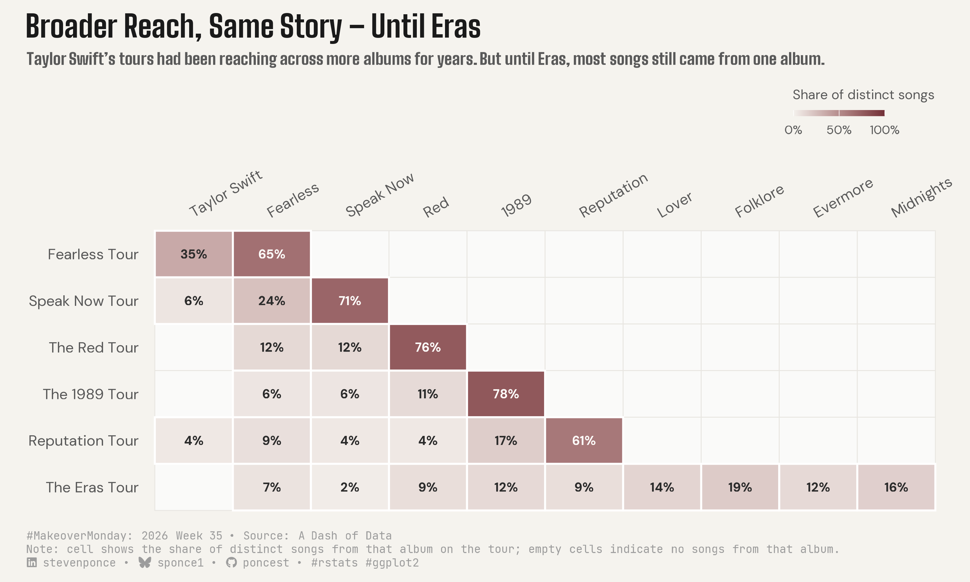
Taylor Swift’s tours had been reaching across more albums for years. But until Eras, most songs still came from one album.

A tour-by-album heatmap shows the share of each Taylor Swift tour’s distinct setlist songs drawn from every album. The albums represented broadened steadily from the Fearless Tour through the Reputation Tour, yet one album still supplied 61-78% of each tour’s songs; only the Eras Tour spread evenly across nine albums, topping out at 19%. Built in R with ggplot2, row-normalized song shares, and a single sequential color scale.

Original

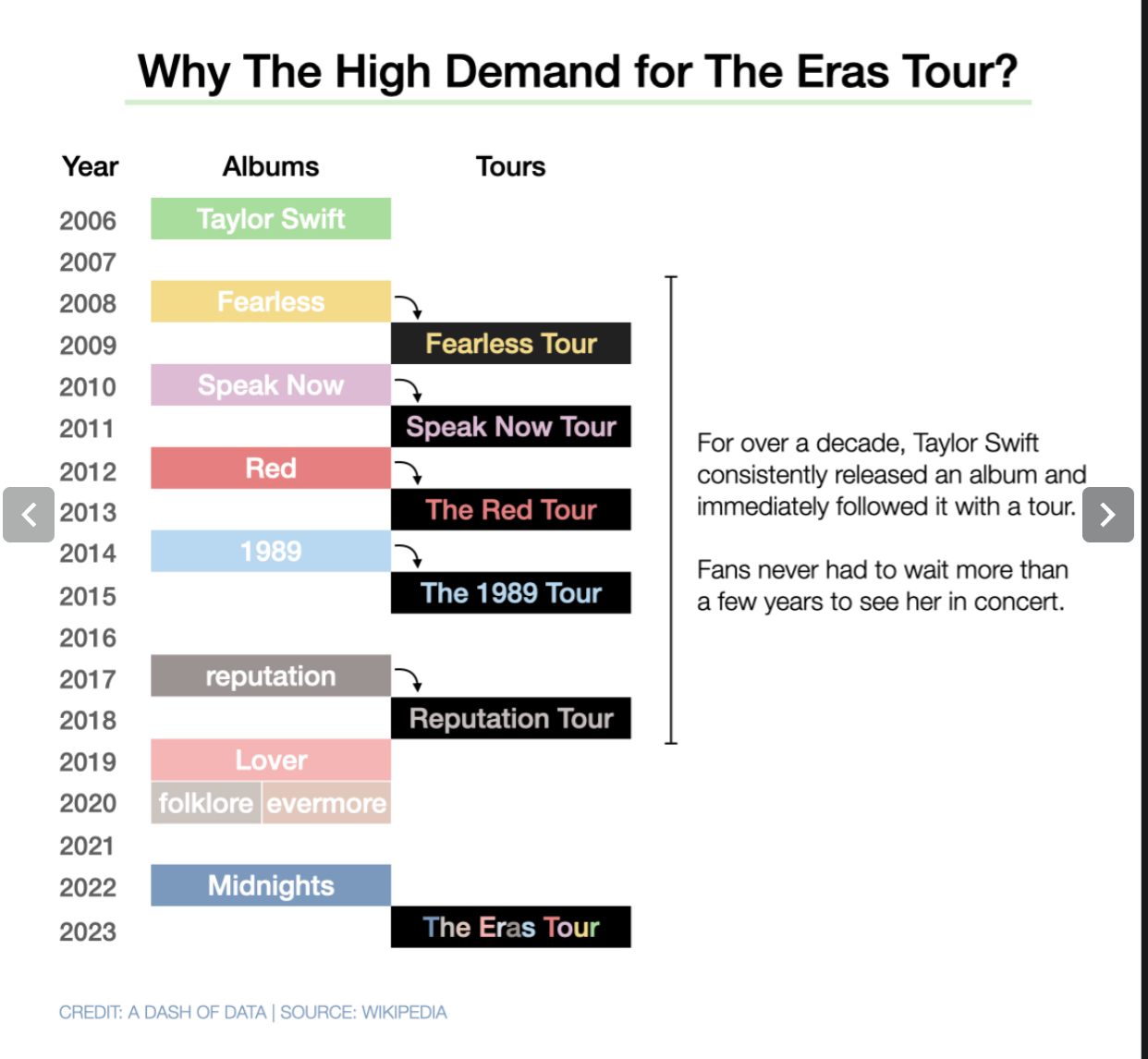
The original visualization comes from Taylor Swift Tours

Original visualization

Makeover

Figure 1: A heatmap titled “Broader Reach, Same Story — Until Eras” showing six Taylor Swift tours, in chronological order top to bottom, by ten studio albums, in chronological release order left to right. Cell color and label show the percentage of songs in that tour’s distinct setlist drawn from each album. For the first five tours, one album dominated, accounting for 61 to 78 percent of songs performed, even as the range of albums represented widened – Fearless 65%, Speak Now 71%, Red 76%, 1989 78%, Reputation 61%. The pattern broke only with the Eras Tour: its top album, Folklore, accounted for just 19% of songs, spread across nine albums represented. The debut album “Taylor Swift” appears in three of the first five tours but has zero songs in the Eras Tour, the only album absent from it. Data from A Dash of Data via the MakeoverMonday 2026 week 35 challenge.

Steps to Create this Graphic

1. Load Packages & Setup

```{r}
#| label: load
#| warning: false
#| message: false      
#| results: "hide"     

## 1. LOAD PACKAGES & SETUP ----
suppressPackageStartupMessages({
  if (!require("pacman")) install.packages("pacman")
  pacman::p_load(
    tidyverse, ggtext, showtext, scales, glue, janitor, ggview
)
})

# Source utility functions
suppressMessages(
  source(here::here("R/utils/fonts.R")))
  source(here::here("R/utils/social_icons.R"))
  source(here::here("R/themes/base_theme.R"))
```

2. Read in the Data

```{r}
#| label: read
#| include: true
#| eval: true
#| warning: false
#| 

df_raw <- readxl::read_excel(
  here::here("data/MakeoverMonday/2026/MM2026_wk35.xlsx"))  |>
  clean_names()
```

3. Examine the Data

```{r}
#| label: examine
#| include: true
#| eval: true
#| results: 'hide'
#| warning: false

glimpse(df_raw)
skimr::skim_without_charts(df_raw)
```

4. Tidy Data

```{r}
#| label: tidy
#| warning: false

# Row for "You Belong with Me" (The Red Tour) carries Speak Now Tour's
# dates (2011-02-09 / 2012-03-18) instead of Red Tour's own
# (2013-03-13 / 2014-06-12) -- confirmed against the other 16 Red Tour
# rows, which are internally consistent.
df_raw <- df_raw |>
  mutate(
    start_date = if_else(
      tour == "The Red Tour", as_datetime("2013-03-13"), start_date
    ),
    end_date = if_else(
      tour == "The Red Tour", as_datetime("2014-06-12"), end_date
    )
  )

### |- chronological ordering ----
tour_levels <- c(
  "Fearless Tour", "Speak Now Tour", "The Red Tour",
  "The 1989 Tour", "Reputation Tour", "The Eras Tour"
)

album_levels <- c(
  "Taylor Swift", "Fearless", "Speak Now", "Red", "1989",
  "Reputation", "Lover", "Folklore", "Evermore", "Midnights"
)

### |- guard against silent level-order corruption ----
album_mismatch <- setdiff(unique(df_raw$album), album_levels)
if (length(album_mismatch) > 0) {
  stop(
    "Album value(s) in data not found in album_levels: ",
    paste(album_mismatch, collapse = ", ")
  )
}

### |- build matrix data ----
matrix_data <- df_raw |>
  mutate(
    tour  = factor(tour, levels = tour_levels),
    album = factor(album, levels = album_levels)
  ) |>
  summarise(
    n_songs = n_distinct(song),
    .by = c(tour, album)
  ) |>
  complete(tour, album, fill = list(n_songs = 0)) |>
  mutate(
    tour_total = sum(n_songs),
    album_share = if_else(tour_total > 0, n_songs / tour_total, 0),
    .by = tour
  )

### |- verification ----
stopifnot(n_distinct(matrix_data$tour) == 6)
stopifnot(n_distinct(matrix_data$album) == 10)
stopifnot(nrow(matrix_data) == 60)
stopifnot(
  matrix_data |>
    summarise(total_share = sum(album_share), .by = tour) |>
    pull(total_share) |>
    (\(x) all(near(x, 1)))()
)

### |- split for layered encoding (explicit absence vs. intensity) ----
zero_data <- matrix_data |> filter(n_songs == 0)
tile_data <- matrix_data |> filter(n_songs > 0)

### |- label every nonzero cell with its share ----
label_data <- tile_data |>
  mutate(label = label_percent(accuracy = 1)(album_share))
```

5. Visualization Parameters

```{r}
#| label: params
#| include: true
#| warning: false

### |- plot aesthetics ----
clrs <- get_theme_colors()

zero_fill_col   <- "#FAFAF9"
zero_border_col <- "#E8E6E1"
label_dark_col  <- "#2B2B2B"
label_light_col <- "#FDFBF9"

### |- titles and caption ----
title_text <- str_glue("Broader Reach, Same Story -- Until Eras")

subtitle_text <- str_glue(
  "Taylor Swift's tours had been reaching across more albums for years. ",
  "But until Eras, most songs still came from one album."
)

caption_text <- create_mm_caption(
  mm_year = 2026,
  mm_week = 35,
  source_text = str_glue(
    "A Dash of Data<br>",
    "Note: cell shows the share of distinct songs from that album on the ",
    "tour; empty cells indicate no songs from that album."
  )
)

### |- typography color hierarchy ----
title_col    <- "#1A1A1A"
subtitle_col <- "#595959"
axis_col     <- "#595959"
caption_col  <- "#9C9C9C"

### |- fonts ----
setup_fonts()
fonts <- get_font_families()

### |- plot theme ----
base_theme <- create_base_theme(clrs)

weekly_theme <- extend_weekly_theme(
  base_theme,
  theme(
    panel.grid = element_blank(),
    axis.ticks = element_blank(),
    axis.text.x = element_text(angle = 30, hjust = 0, vjust = 0, color = axis_col),
    axis.text.y = element_text(hjust = 1, color = axis_col),
    legend.position = "top",
    legend.justification = "right",
    legend.title = element_text(size = rel(0.7), color = axis_col),
    legend.text = element_text(size = rel(0.65), color = axis_col),
    legend.key.width = unit(0.8, "cm"),
    legend.key.height = unit(0.18, "cm"),
    plot.title = element_textbox_simple(
      size = rel(1.6), face = "bold", color = title_col,
      margin = margin(b = 6), family = fonts$title_1
    ),
    plot.subtitle = element_textbox_simple(
      size = rel(0.85), color = subtitle_col,
      margin = margin(b = 8), family = fonts$title_1
    ),
    plot.caption = element_textbox_simple(
      size = rel(0.6), color = caption_col,
      margin = margin(t = 12), family = fonts$caption
    )
  )
)

theme_set(weekly_theme)
```

6. Plot

```{r}
#| label: plot
#| warning: false

### |- plot ----
p <- matrix_data |>
  ggplot(aes(x = album, y = tour)) +
  geom_tile(
    data = zero_data,
    fill = zero_fill_col,
    color = zero_border_col,
    linewidth = 0.3
  ) +
  geom_tile(
    data = tile_data,
    aes(fill = album_share),
    color = "white",
    linewidth = 0.7
  ) +
  geom_text(
    data = label_data,
    aes(
      label = label,
      color = album_share >= 0.5
    ),
    size = 3.3,
    family = fonts$text,
    fontface = "bold",
    show.legend = FALSE
  ) +
  scale_x_discrete(position = "top", limits = album_levels) +
  scale_y_discrete(limits = rev(tour_levels)) +
  scale_fill_gradient(
    low = "#F4F1ED", high = "#722F37",
    limits = c(0, 1), breaks = c(0, 0.5, 1),
    labels = label_percent(accuracy = 1),
    name = "Share of distinct songs",
    guide = guide_colorbar(
      title.position = "top", title.hjust = 0,
      barwidth = unit(2.4, "cm"), barheight = unit(0.16, "cm")
    )
  ) +
  scale_color_manual(
    values = c(`TRUE` = label_light_col, `FALSE` = label_dark_col)
  ) +
  labs(
    title = title_text,
    subtitle = subtitle_text,
    caption = caption_text,
    x = NULL, y = NULL
  ) +
  coord_cartesian(clip = "off")
```

7. Save

```{r}
#| label: save
#| warning: false

### |- save ----
main_path  <- here::here("data_visualizations", "MakeoverMonday", "2026", "mm_2026_35.png")
thumb_path <- here::here("data_visualizations", "MakeoverMonday", "2026", "thumbnails", "mm_2026_35.png")

# Full-size version, for the QMD figure
save_ggplot(
  plot = p,
  file = main_path,
  width = 10,
  height = 6,
  units = "in",
  dpi = 320,
  create.dir = TRUE
)

# Reduced-size thumbnail, for the YAML `image:` field
fs::dir_create(dirname(thumb_path))
magick::image_read(main_path) |>
  magick::image_resize("400") |>
  magick::image_write(thumb_path)
```

8. Session Info

TipExpand for Session Info

R version 4.6.1 (2026-06-24)
Platform: aarch64-apple-darwin23
Running under: macOS Tahoe 26.6.2

Matrix products: default
BLAS:   /Library/Frameworks/R.framework/Versions/4.6/Resources/lib/libRblas.0.dylib 
LAPACK: /Library/Frameworks/R.framework/Versions/4.6/Resources/lib/libRlapack.dylib;  LAPACK version 3.12.1

locale:
[1] en_US.UTF-8/en_US.UTF-8/en_US.UTF-8/C/en_US.UTF-8/en_US.UTF-8

time zone: America/New_York
tzcode source: internal

attached base packages:
[1] stats     graphics  grDevices utils     datasets  methods   base     

other attached packages:
 [1] here_1.0.2      ggview_0.2.2    janitor_2.2.1   glue_1.8.1     
 [5] scales_1.4.0    showtext_0.9-8  showtextdb_3.0  sysfonts_0.8.9 
 [9] ggtext_0.1.2    lubridate_1.9.5 forcats_1.0.1   stringr_1.6.0  
[13] dplyr_1.2.1     purrr_1.2.2     readr_2.2.0     tidyr_1.3.2    
[17] tibble_3.3.1    ggplot2_4.0.3   tidyverse_2.0.0 pacman_0.5.1   

loaded via a namespace (and not attached):
 [1] gtable_0.3.6       xfun_0.60          htmlwidgets_1.6.4  tzdb_0.5.0        
 [5] vctrs_0.7.3        tools_4.6.1        generics_0.1.4     curl_7.1.0        
 [9] pkgconfig_2.0.3    RColorBrewer_1.1-3 skimr_2.2.2        S7_0.2.2          
[13] readxl_1.5.0       lifecycle_1.0.5    compiler_4.6.1     farver_2.1.2      
[17] textshaping_1.0.5  repr_1.1.7         codetools_0.2-20   snakecase_0.11.1  
[21] litedown_0.10      htmltools_0.5.9    yaml_2.3.12        pillar_1.11.1     
[25] magick_2.9.1       commonmark_2.0.0   tidyselect_1.2.1   digest_0.6.39     
[29] stringi_1.8.7      rprojroot_2.1.1    fastmap_1.2.0      grid_4.6.1        
[33] cli_3.6.6          magrittr_2.0.5     base64enc_0.1-6    withr_3.0.3       
[37] timechange_0.4.0   rmarkdown_2.31     otel_0.2.0         cellranger_1.1.0  
[41] ragg_1.5.2         hms_1.1.4          evaluate_1.0.5     knitr_1.51        
[45] haven_2.5.5        markdown_2.0       rlang_1.3.0        gridtext_0.1.6    
[49] Rcpp_1.1.2         xml2_1.6.0         rstudioapi_0.19.0  jsonlite_2.0.0    
[53] R6_2.6.1           fs_2.1.0           systemfonts_1.3.2 

9. GitHub Repository

TipExpand for GitHub Repo

The complete code for this analysis is available in mm_2026_35.qmd.

For the full repository, click here.

10. References

TipExpand for References

Primary Data (Makeover Monday): 1. Makeover Monday 2026 Week 35: Taylor Swift Tours - Excel: 135 rows × 5 columns (tour, start_date, end_date, album, song). Song-level setlist data across Taylor Swift’s six headlining tours (Fearless Tour through The Eras Tour), with each row’s album identifying which of her ten studio albums that song originally came from. One row (The Red Tour, “You Belong with Me”) carries Speak Now Tour’s date range in the source file rather than Red Tour’s own; corrected in Section 4 (Tidy Data) prior to analysis. - The original visualization plots album release years against tour years (2006–2023) to argue that Taylor Swift “never made fans wait” — pairing each album with its supporting tour in sequence. That framing describes release cadence, a variable this dataset doesn’t actually contain (no album release dates, only tour date ranges). This makeover abandons the cadence argument and encodes what the data actually supports: each tour’s setlist as a share of songs per album. The resulting heatmap shows the range of albums performed broadening tour over tour, while one album still supplied 61–78% of the setlist through the Reputation Tour — only The Eras Tour spread evenly across nine albums, topping out at 19% for its top contributor, Folklore. Source Data: 2. A Dash of Data, 2023, A Data Scientist Breaks Down All 10 Taylor Swift Albums (The Extended Version)

11. Custom Functions Documentation

Note📦 Custom Helper Functions

This analysis uses custom functions from my personal module library for efficiency and consistency across projects.

Functions Used:

• fonts.R: setup_fonts(), get_font_families() - Font management with showtext
• social_icons.R: create_social_caption() - Generates formatted social media captions
• image_utils.R: save_plot() - Consistent plot saving with naming conventions
• base_theme.R: create_base_theme(), extend_weekly_theme(), get_theme_colors() - Custom ggplot2 themes

Why custom functions?
These utilities standardize theming, fonts, and output across all my data visualizations. The core analysis (data tidying and visualization logic) uses only standard tidyverse packages.

Source Code:
View all custom functions → GitHub: R/utils