SEC Roster Budgets Run Deeper Than Any Other Power Conference’s

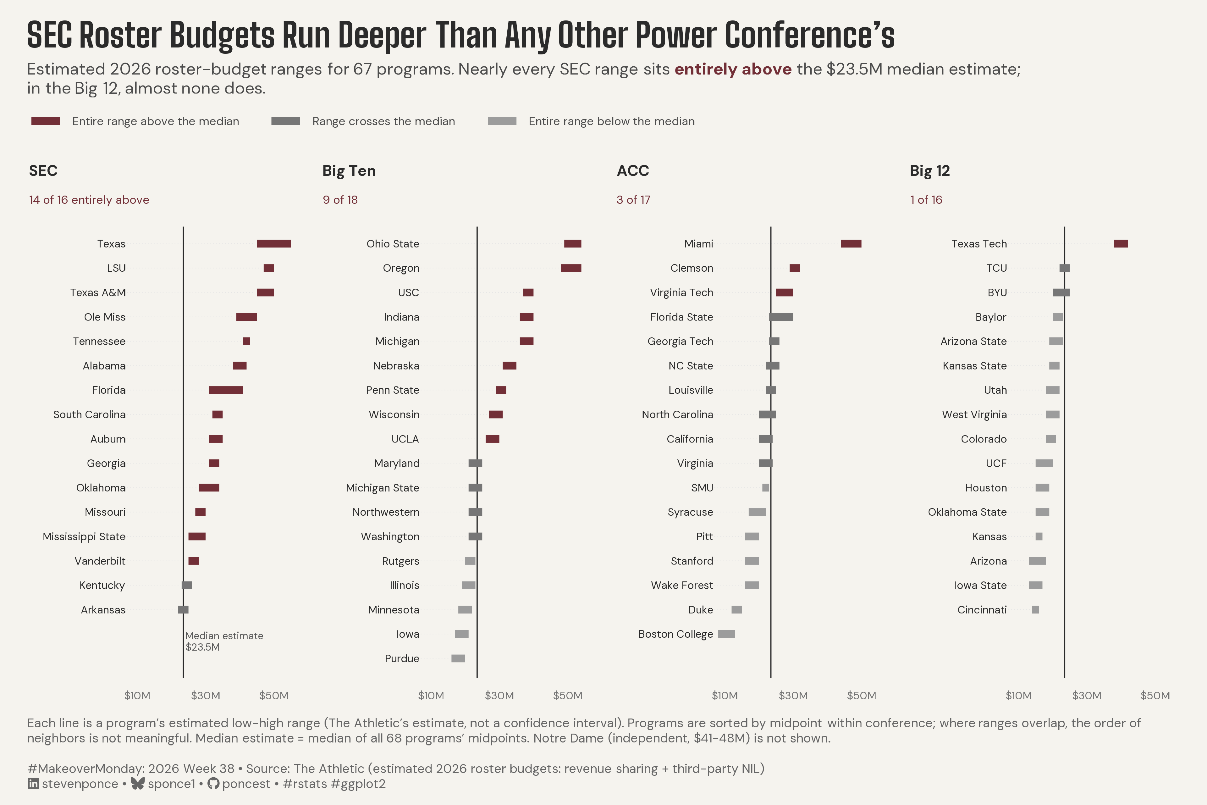
Estimated 2026 roster-budget ranges for 67 programs. Nearly every SEC range sits entirely above the $23.5M median estimate; in the Big 12, almost none does.

Estimated 2026 roster-budget ranges for 67 programs show 14 of 16 SEC ranges entirely above the $23.5M median, versus 1 of 16 in the Big 12. Each Athletic estimate is kept as a low-high range and classified against the median of all 68 midpoints. Built with R, ggplot2 and ggtext.

Original

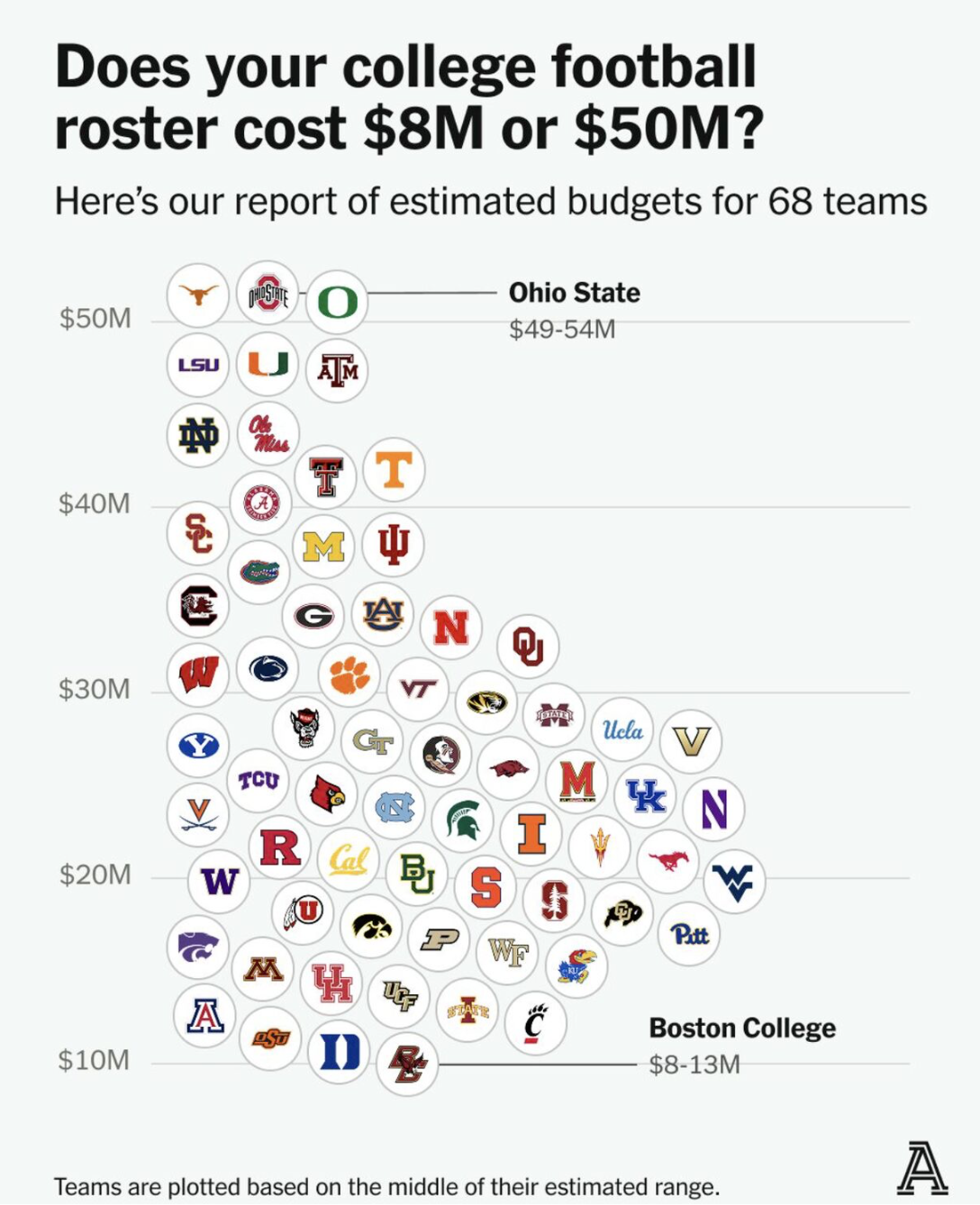
The original visualization comes from CFB Roster Spending 2026

Original visualization

Makeover

Figure 1: Range chart in four panels, titled SEC Roster Budgets Run Deeper Than Any Other Power Conference’s. 14 of 16 SEC programs’ estimated 2026 roster-budget ranges sit entirely above the $23.5M median, versus 9 of 18 in the Big Ten, 3 of 17 in the ACC, and 1 of 16 in the Big 12. Each bar spans one program’s low-to-high estimate: burgundy if entirely above the median line, dark gray if it crosses the line, light gray if entirely below. Texas Tech is the only Big 12 program above the line. Source: The Athletic.

Steps to Create this Graphic

1. Load Packages & Setup

```{r}
#| label: load
#| warning: false
#| message: false      
#| results: "hide"     

## 1. LOAD PACKAGES & SETUP ----
suppressPackageStartupMessages({
  if (!require("pacman")) install.packages("pacman")
  pacman::p_load(
    tidyverse, ggtext, showtext, scales, glue, 
  janitor, ggview
)
})

# Source utility functions
suppressMessages(
  source(here::here("R/utils/fonts.R")))
  source(here::here("R/utils/social_icons.R"))
  source(here::here("R/themes/base_theme.R"))

### |- figure size ----
fig_w <- 12
fig_h <- 8
```

2. Read in the Data

```{r}
#| label: read
#| include: true
#| eval: true
#| warning: false
#| 

df_raw <- read_csv(
  here::here("data/MakeoverMonday/2026/cfb_roster_budgets_2026.csv"))  |>
  clean_names()
```

3. Examine the Data

```{r}
#| label: examine
#| include: true
#| eval: true
#| results: 'hide'
#| warning: false

glimpse(df_raw)
skimr::skim_without_charts(df_raw)
```

4. Tidy Data

```{r}
#| label: tidy
#| warning: false

### |- reference line ----
# Median of all 68 midpoints (Notre Dame included in the benchmark)
nat_median <- median(df_raw$est_mid_musd)

### |- classify each estimated range against the line ----
# Uses the WHOLE range, not the midpoint:
#   above = low end is above the line
#   below = high end is below the line
#   straddles = the line falls inside the range
conf_levels <- c("SEC", "Big Ten", "ACC", "Big 12")

plot_data <- df_raw |>
  filter(conference != "Independent") |>
  mutate(
    state = case_when(
      est_low_musd > nat_median ~ "above",
      est_high_musd < nat_median ~ "below",
      .default = "straddles"
    ),
    state = factor(state, levels = c("above", "straddles", "below")),
    conference = factor(conference, levels = conf_levels)
  ) |>
  arrange(conference, desc(est_mid_musd), desc(est_high_musd), team) |>
  mutate(row = row_number(), .by = conference)

panel_stats <- plot_data |>
  summarise(
    n = n(),
    n_above = sum(state == "above"),
    n_below = sum(state == "below"),
    .by = conference
  ) |>
  arrange(conference) |>
  mutate(count_label = if_else(
    row_number() == 1,
    paste0(n_above, " of ", n, " entirely above"),
    paste0(n_above, " of ", n)
  ))

nd <- df_raw |> filter(conference == "Independent")
```

5. Visualization Parameters

```{r}
#| label: params
#| include: true
#| warning: false

### |- plot aesthetics ----
col_above <- "#722F37"
col_straddle <- "#767676"
col_below <- "#9C9C9C"
col_ink <- "#2B2B2B"

colors <- get_theme_colors(
  palette = list(
    primary      = col_above,
    neutral_dark = col_straddle,
    neutral_mid  = col_below
  )
)
clrs <- colors$palette

### |- layout constants (data units) ----
x_names <- 6.5
x_head <- -21.5
x_lim <- c(-22, 57)
y_lim <- c(19, -2.6)

### |- titles and caption ----
title_text <- "SEC Roster Budgets Run Deeper Than Any Other Power Conference's" 

subtitle_text <- str_glue(
  "Estimated 2026 roster-budget ranges for 67 programs. Nearly every SEC range sits ",
  "<span style='color:{col_above}'><b>entirely above</b></span> ",
  "the ${nat_median}M median estimate;<br>in the Big 12, almost none does."
)

caption_text <- create_mm_caption(
  mm_year = 2026,
  mm_week = 38,
  source_text = "The Athletic (estimated 2026 roster budgets: revenue sharing + third-party NIL)"
)

note_text <- str_glue(
  "Each line is a program's estimated low-high range (The Athletic's estimate, not a confidence interval). ",
  "Programs are sorted by midpoint within conference; where ranges overlap, the order of neighbors is not meaningful. ",
  "Median estimate = median of all 68 programs' midpoints. ",
  "{nd$team} (independent, {nd$budget_label}) is not shown."
)

caption_full <- str_glue("{note_text}<br><br>{caption_text}")


### |- fonts ----
setup_fonts()
fonts <- get_font_families()

### |- plot theme ----
base_theme <- create_base_theme(colors)

weekly_theme <- extend_weekly_theme(
  base_theme,
  theme(
    plot.title = element_textbox_simple(
      family = fonts$title_1, face = "bold", size = rel(1.7), colour = col_ink,
      width = unit(1, "npc"), margin = margin(b = 6)
    ),
    plot.subtitle = element_textbox_simple(
      family = fonts$text, size = rel(0.85), colour = "grey30",
      width = unit(1, "npc"), lineheight = 1.15, margin = margin(b = 12)
    ),
    plot.caption = element_textbox_simple(
      family = fonts$text, size = rel(0.65), colour = "grey40",
      width = unit(1, "npc"), lineheight = 1.2, margin = margin(t = 12)
    ),
    plot.title.position = "plot",
    plot.caption.position = "plot",
    strip.text = element_blank(),
    axis.text.y = element_blank(),
    axis.ticks = element_blank(),
    axis.title = element_blank(),
    axis.text.x = element_text(family = fonts$text, size = rel(0.7), colour = "grey45"),
    panel.grid = element_blank(),
    panel.spacing.x = unit(0.6, "cm"),
    legend.position = "top",
    legend.justification = "left",
    legend.location = "plot",
    legend.title = element_blank(),
    legend.background = element_blank(),
    legend.key = element_blank(),
    legend.key.width = unit(0.9, "cm"),
    legend.key.height = unit(0.35, "cm"),
    legend.key.spacing.x = unit(0.7, "cm"),
    legend.text = element_text(family = fonts$text, size = rel(0.6), colour = "grey30"),
    legend.margin = margin(0, 0, 0, 0),
    legend.box.margin = margin(b = 6),
    plot.margin = margin(15, 20, 10, 20)
  )
)

theme_set(weekly_theme)
```

6. Plot

```{r}
#| label: plot
#| warning: false

### |- reference-line label + line span ----
median_label <- tibble(
  conference = factor("SEC", levels = conf_levels),
  x = nat_median + 0.8,
  y = 17.3,
  label = paste0("Median estimate\n$", nat_median, "M")
)

# One segment per panel
median_line <- tibble(conference = factor(conf_levels, levels = conf_levels))

### |- plot ----
p <- ggplot(plot_data) +
  geom_segment(
    data = \(d) filter(d, est_low_musd - 0.7 > x_names + 0.5),
    aes(x = x_names + 0.5, xend = est_low_musd - 0.7, y = row, yend = row),
    colour = "grey90", linewidth = 0.25, linetype = "dotted"
  ) +
  geom_segment(
    data = median_line,
    aes(x = nat_median, xend = nat_median, y = 0.3, yend = 18.8),
    inherit.aes = FALSE, colour = col_ink, linewidth = 0.4
  ) +
  geom_segment(
    aes(x = est_low_musd, xend = est_high_musd, y = row, yend = row, colour = state),
    linewidth = 2.6, lineend = "butt"
  ) +
  geom_text(
    aes(x = x_names, y = row, label = team),
    hjust = 1, size = 2.7, family = fonts$text, colour = col_ink
  ) +
  geom_text(
    data = panel_stats,
    aes(x = x_head, y = -2, label = conference),
    hjust = 0, size = 3.8, fontface = "bold", family = fonts$text, colour = col_ink
  ) +
  geom_text(
    data = panel_stats,
    aes(x = x_head, y = -0.8, label = count_label),
    hjust = 0, size = 2.9, family = fonts$text, colour = col_above
  ) +
  geom_text(
    data = median_label,
    aes(x = x, y = y, label = label),
    hjust = 0, size = 2.5, lineheight = 0.95, family = fonts$text, colour = "grey35"
  ) +
  scale_colour_manual(
    values = c(above = col_above, straddles = col_straddle, below = col_below),
    labels = c(
      above     = "Entire range above the median",
      straddles = "Range crosses the median",
      below     = "Entire range below the median"
    )
  ) +
  guides(colour = guide_legend(override.aes = list(linewidth = 2.6))) +
  scale_x_continuous(
    limits = x_lim, breaks = c(10, 30, 50),
    labels = \(x) str_c("$", x, "M"), expand = expansion(0)
  ) +
  scale_y_reverse(limits = y_lim, expand = expansion(0)) +
  facet_wrap(~conference, nrow = 1) +
  labs(title = title_text, subtitle = subtitle_text, caption = caption_full)
```

7. Save

```{r}
#| label: save
#| warning: false

### |- save ----
main_path  <- here::here("data_visualizations", "MakeoverMonday", "2026", "mm_2026_38.png")
thumb_path <- here::here("data_visualizations", "MakeoverMonday", "2026", "thumbnails", "mm_2026_38.png")

# Full-size version, for the QMD figure
save_ggplot(
  plot = p,
  file = main_path,
  width = fig_w, height = fig_h,
  units = "in", dpi = 320,
  create.dir = TRUE
)

# Reduced-size thumbnail, for the YAML `image:` field
fs::dir_create(dirname(thumb_path))
magick::image_read(main_path) |>
  magick::image_resize("400") |>
  magick::image_write(thumb_path)
```

8. Session Info

TipExpand for Session Info

R version 4.6.1 (2026-06-24)
Platform: aarch64-apple-darwin23
Running under: macOS Tahoe 26.6.2

Matrix products: default
BLAS:   /Library/Frameworks/R.framework/Versions/4.6/Resources/lib/libRblas.0.dylib 
LAPACK: /Library/Frameworks/R.framework/Versions/4.6/Resources/lib/libRlapack.dylib;  LAPACK version 3.12.1

locale:
[1] en_US.UTF-8/en_US.UTF-8/en_US.UTF-8/C/en_US.UTF-8/en_US.UTF-8

time zone: America/New_York
tzcode source: internal

attached base packages:
[1] stats     graphics  grDevices utils     datasets  methods   base     

other attached packages:
 [1] here_1.0.2      ggview_0.2.2    janitor_2.2.1   glue_1.8.1     
 [5] scales_1.4.0    showtext_0.9-8  showtextdb_3.0  sysfonts_0.8.9 
 [9] ggtext_0.2.0    lubridate_1.9.5 forcats_1.0.1   stringr_1.6.0  
[13] dplyr_1.2.1     purrr_1.2.2     readr_2.2.0     tidyr_1.3.2    
[17] tibble_3.3.1    ggplot2_4.0.3   tidyverse_2.0.0 pacman_0.5.1   

loaded via a namespace (and not attached):
 [1] gtable_0.3.6       xfun_0.60          htmlwidgets_1.6.4  tzdb_0.5.0        
 [5] vctrs_0.7.3        tools_4.6.1        generics_0.1.4     curl_7.1.0        
 [9] parallel_4.6.1     pkgconfig_2.0.3    RColorBrewer_1.1-3 skimr_2.2.2       
[13] S7_0.2.2           lifecycle_1.0.5    compiler_4.6.1     farver_2.1.2      
[17] textshaping_1.0.5  repr_1.1.7         codetools_0.2-20   snakecase_0.11.1  
[21] litedown_0.10      htmltools_0.5.9    yaml_2.3.12        pillar_1.11.1     
[25] crayon_1.5.3       magick_2.9.1       commonmark_2.0.0   tidyselect_1.2.1  
[29] digest_0.6.39      stringi_1.8.7      labeling_0.4.3     rprojroot_2.1.1   
[33] fastmap_1.2.0      grid_4.6.1         cli_3.6.6          magrittr_2.0.5    
[37] base64enc_0.1-6    withr_3.0.3        bit64_4.8.2        timechange_0.4.0  
[41] rmarkdown_2.31     bit_4.6.0          otel_0.2.0         ragg_1.5.2        
[45] hms_1.1.4          evaluate_1.0.5     knitr_1.51         markdown_2.0      
[49] rlang_1.3.0        gridtext_0.1.6     Rcpp_1.1.2         xml2_1.6.0        
[53] rstudioapi_0.19.0  vroom_1.7.1        jsonlite_2.0.0     R6_2.6.1          
[57] fs_2.1.0           systemfonts_1.3.2 

9. GitHub Repository

TipExpand for GitHub Repo

The complete code for this analysis is available in mm_2026_38.qmd.

For the full repository, click here.

10. References

TipExpand for References

Primary Data (Makeover Monday): 1. Makeover Monday 2026 Week 38: Does your college football roster cost $8M or $50M? - CSV: 68 rows × 9 columns (spend_rank, team, conference, est_low_musd, est_high_musd, est_mid_musd, range_width_musd, budget_label, ap_rank). Estimated 2026 roster budgets in millions of USD, reported by The Athletic as a low–high range per program and covering the total money available to assemble a roster, including revenue sharing and third-party NIL. These are estimates, not disclosed financials, and are treated here as reported estimate bands, not statistical confidence intervals. Ranges are $2M–$10M wide (median $4M). The source file’s description reads “68 Power 4 programs plus Notre Dame,” but the CSV itself contains 68 rows in total: 67 programs across the SEC (16), Big Ten (18), ACC (17) and Big 12 (16), plus Notre Dame as the only Independent, which is consistent with the original’s “68 teams.” ap_rank is populated for 25 of 68 programs (blank means unranked) and is not used in this makeover. - The original visualization stacks all 68 programs as team logos by the midpoint of each estimated range on a $10M–$50M axis. Only two programs are labeled (Ohio State, $49–54M; Boston College, $8–13M), so the ranges are visible for those two only, and identifying most teams depends on recognizing logos. This makeover keeps every program’s low–high range visible, names each program, groups programs by conference, and classifies each range against one reference line: the median of all 68 midpoints ($23.5M). The result is a clear gradient in how many ranges sit entirely above that line: SEC 14 of 16 (none entirely below), Big Ten 9 of 18, ACC 3 of 17, and Big 12 1 of 16 (13 entirely below). The gradient holds at $20M and $30M reference lines (at $30M, 10/6/1/1, where the ACC and Big 12 tie), with leave-one-conference-out medians (the SEC still has 15 of 16 above its outside median of $22M), and using midpoints alone (16/9/7/2 at or above the median). Programs are sorted by midpoint within each conference for readability only; where ranges overlap, the order of neighbors is not meaningful. Notre Dame (independent, $41–48M) is omitted from the panels because it is a one-team group, and it is included in the median.

Source Data: 2. The Athletic, 2026, College football roster-budget estimates (interactive) 3. Sagers, R., 2026, LinkedIn post on The Athletic’s roster-budget report 4. Dataset (CSV): cfb_roster_budgets_2026.csv

11. Custom Functions Documentation

Note📦 Custom Helper Functions

This analysis uses custom functions from my personal module library for efficiency and consistency across projects.

Functions Used:

• fonts.R: setup_fonts(), get_font_families() - Font management with showtext
• social_icons.R: create_social_caption() - Generates formatted social media captions
• image_utils.R: save_plot() - Consistent plot saving with naming conventions
• base_theme.R: create_base_theme(), extend_weekly_theme(), get_theme_colors() - Custom ggplot2 themes

Why custom functions?
These utilities standardize theming, fonts, and output across all my data visualizations. The core analysis (data tidying and visualization logic) uses only standard tidyverse packages.

Source Code:
View all custom functions → GitHub: R/utils