Most cowbell comes one song at a time

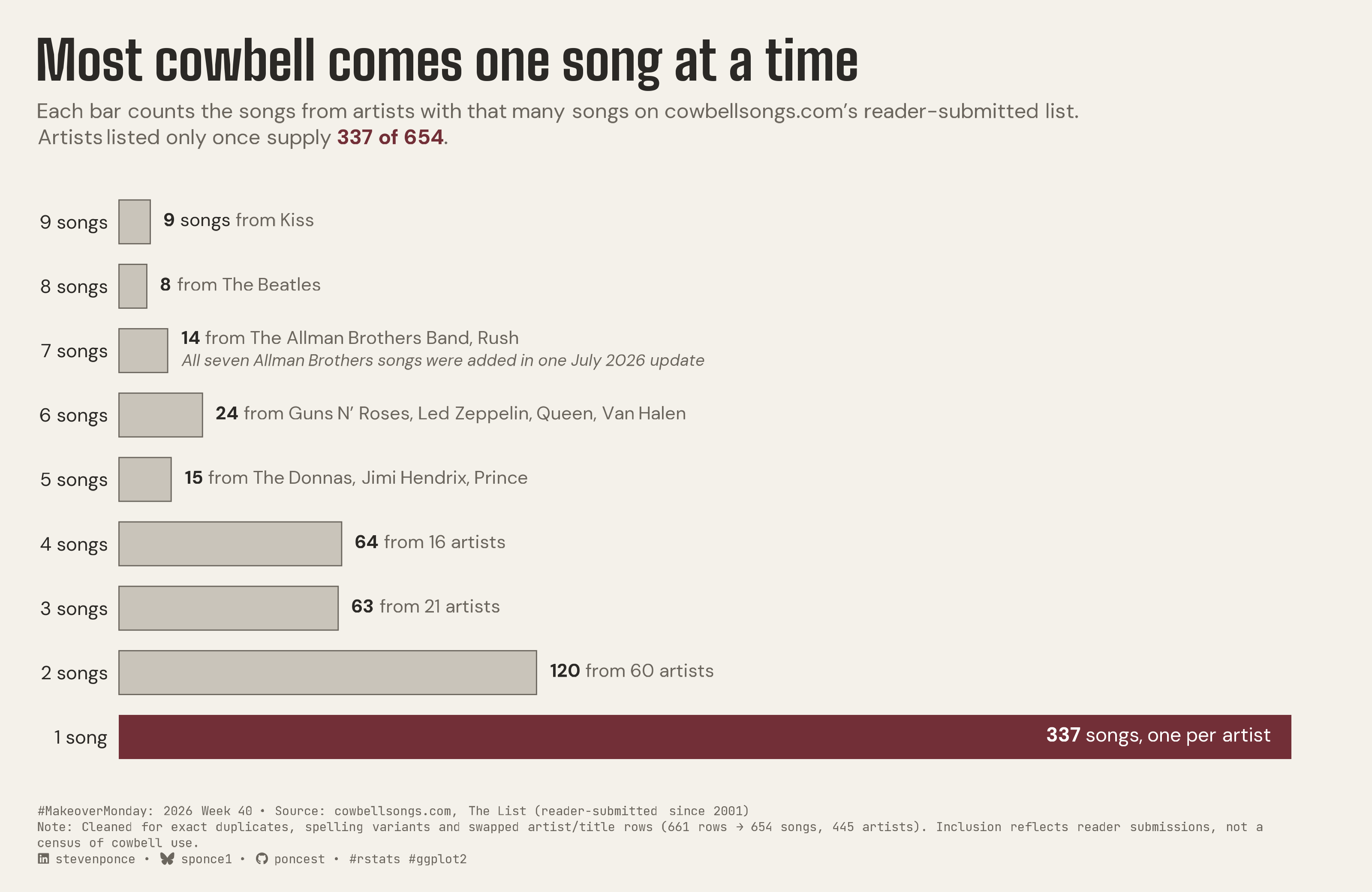
Each bar counts the songs from artists with that many songs on cowbellsongs.com’s reader-submitted list. Artists listed only once supply 337 of 654.

A makeover of a cowbell-song leaderboard showing that artists listed only once supply 337 of the 654 songs on cowbellsongs.com’s reader-submitted list. Instead of ranking artists, each bar totals the songs contributed by artists with the same number of songs, after removing duplicates and name variants. Built in R with ggplot2, ggtext, and showtext.

Original

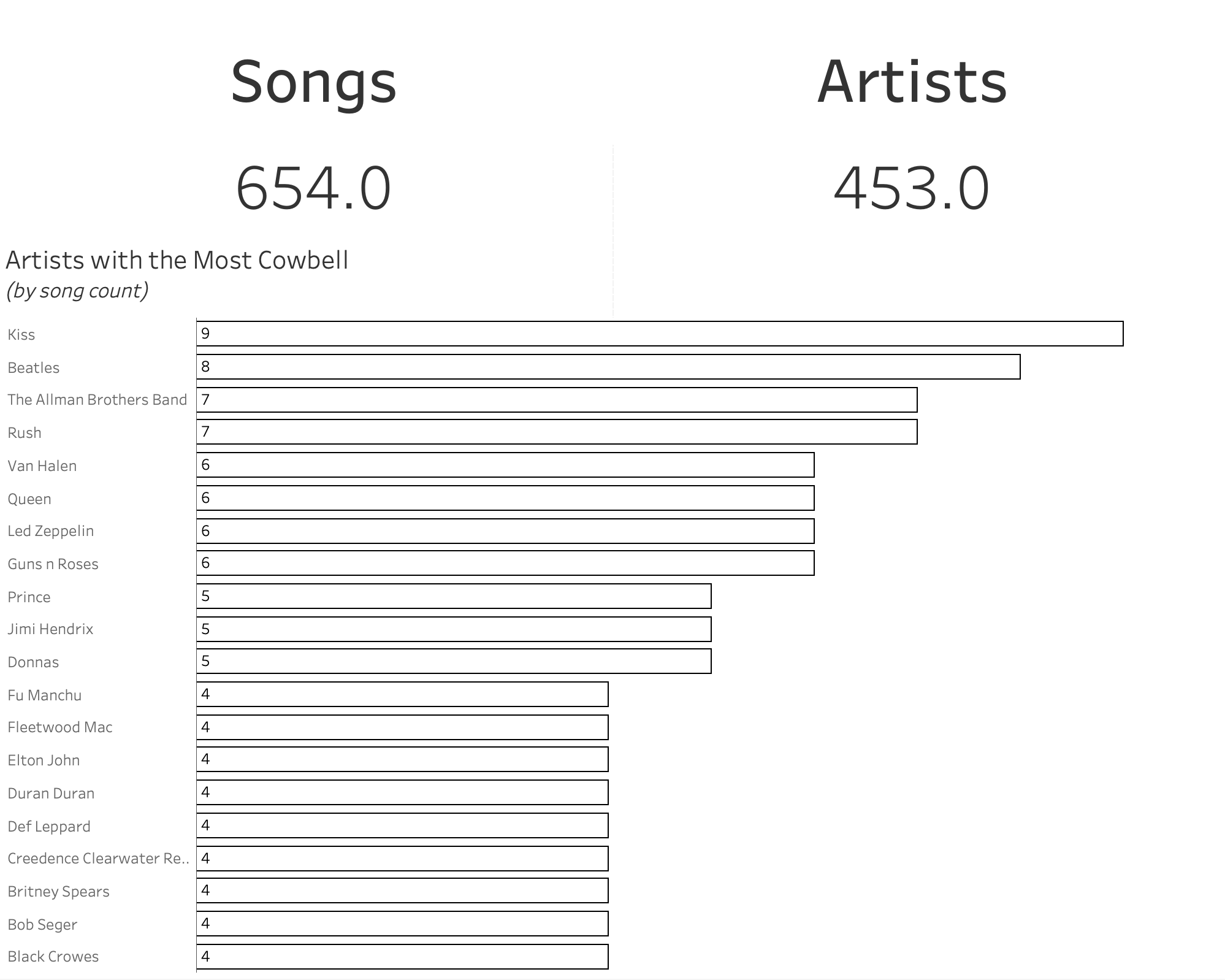
The original visualization comes from Songs with Cowbell

Original visualization

Makeover

Figure 1: Horizontal bar chart titled “Most cowbell comes one song at a time.” It groups the 654 songs on cowbellsongs.com’s reader-submitted list by how many songs each artist has there, and each bar counts the songs that group contributes. The highlighted bottom bar shows that artists listed only once supply 337 songs, just over half the list, one per artist. Above it, gray bars show 9 songs from Kiss, 8 from The Beatles, 14 from The Allman Brothers Band and Rush, 24 from Guns N’ Roses, Led Zeppelin, Queen and Van Halen, and 15 from The Donnas, Jimi Hendrix and Prince, then 64 songs from 16 artists with four each, 63 from 21 artists with three, and 120 from 60 artists with two. A note says all seven Allman Brothers songs were added in one July 2026 update. Source: cowbellsongs.com.

Steps to Create this Graphic

1. Load Packages & Setup

```{r}
#| label: load
#| warning: false
#| message: false      
#| results: "hide"     

## 1. LOAD PACKAGES & SETUP ----
suppressPackageStartupMessages({
  if (!require("pacman")) install.packages("pacman")
  pacman::p_load(
    tidyverse, ggtext, showtext, scales, glue, 
  janitor, ggview, readxl
)
})

# Source utility functions
suppressMessages(
  source(here::here("R/utils/fonts.R")))
  source(here::here("R/utils/social_icons.R"))
  source(here::here("R/themes/base_theme.R"))

### |- figure size ----
fig_w <- 10
fig_h <- 6.5
```

2. Read in the Data

```{r}
#| label: read
#| include: true
#| eval: true
#| warning: false
#| 

df_raw <- readxl::read_excel(
  here::here("data/MakeoverMonday/2026/MM2026_wk40.xlsx"))  |>
  clean_names()
```

3. Examine the Data

```{r}
#| label: examine
#| include: true
#| eval: true
#| results: 'hide'
#| warning: false

glimpse(df_raw)
skimr::skim_without_charts(df_raw)
```

4. Tidy Data

```{r}
#| label: tidy
#| warning: false

### |- cleaning ----
artist_fixes <- c(
  "Jimmy Buffet"                   = "Jimmy Buffett",
  "Sleater Kinney"                 = "Sleater-Kinney",
  "B’52s"                          = "B-52s",
  "Chambers Brothers"              = "The Chambers Brothers",
  "Earth, Wind, and Fire"          = "Earth Wind and Fire",
  "Rage Against the Machine"       = "Rage Against The Machine",
  "Bachman Turner Overdrive (BTO)" = "BTO",
  "Dave Mathews Band"              = "Dave Matthews Band"
)

df_clean <- df_raw |>
  mutate(
    swap    = artist %in% c("The Tide is high", "Deliverance"),
    artist2 = if_else(swap, title, artist),
    title   = if_else(swap, artist, title),
    artist  = artist2
  ) |>
  select(-swap, -artist2) |>
  mutate(
    artist = recode(artist, !!!artist_fixes),
    title = case_when(
      title == "Ain’t Seen Nothing Yet" ~ "You Ain’t Seen Nothing Yet!",
      title == "Time Has Come" ~ "Time Has Come Today",
      .default = title
    )
  ) |>
  distinct(artist, title)

### |- tiers: songs contributed by artists with N songs on the list ----
# display-only name fixes for the named head tiers
display_names <- c(
  "Beatles"      = "The Beatles",
  "Guns n Roses" = "Guns N’ Roses",
  "Donnas"       = "The Donnas"
)

tiers <- df_clean |>
  count(artist, name = "per_artist") |>
  mutate(artist = recode(artist, !!!display_names)) |>
  summarise(
    n_artists = n(),
    songs = sum(per_artist),
    names = str_flatten_comma(artist[order(str_remove(artist, "^The "))]),
    .by = per_artist
  ) |>
  arrange(per_artist)

### |- copy numbers, built from the data ----
n_songs <- sum(tiers$songs)
n_artists <- sum(tiers$n_artists)
t1 <- tiers |> filter(per_artist == 1)
share_t1 <- t1$songs / n_songs
```

5. Visualization Parameters

```{r}
#| label: params
#| include: true
#| warning: false

#### |- plot aesthetics ----
# encoding colors as plain constants 
col_paper <- "#f4f1ea"
col_accent <- "#722F37"
col_bar <- "#c9c4ba"
col_ink <- "#2b2926"
col_muted <- "#6b665e"

clrs <- get_theme_colors(
  palette = list(accent = col_accent, paper = col_paper)
)

### |-  plot data ----
allman_note <- glue(
  "<br><span style='font-size:8.5pt;color:{col_muted};'><i>",
  "All seven Allman Brothers songs were added in one July 2026 update</i></span>"
)

plot_df <- tiers |>
  mutate(
    row_lab = if_else(per_artist == 1, "1 song", glue("{per_artist} songs")),
    row_lab = fct_reorder(row_lab, per_artist), # 9 at top, 1 at bottom
    is_focus = per_artist == 1,
    who = case_when(
      is_focus ~ "one per artist",
      n_artists <= 4 ~ names,
      .default = glue("{n_artists} artists")
    ),
    note = if_else(per_artist == 7, allman_note, ""),
    bar_lab = if_else(
      is_focus,
      glue("<b>{songs}</b> songs, {who}"),
      glue(
        "<b>{songs}</b>{if_else(per_artist == max(per_artist), ' songs', '')}",
        "<span style='color:{col_muted};'> from {who}</span>{note}"
      )
    )
  )

### |-  titles and caption ----
title_text <- "Most cowbell comes one song at a time"

subtitle_text <- glue(
  "Each bar counts the songs from artists with that many songs on ",
  "cowbellsongs.com's reader-submitted list.<br>Artists listed only once supply ",
  "<span style='color:{col_accent};'><b>{t1$songs} of {n_songs}</b></span>."
)

caption_text <- create_mm_caption(
  mm_year = 2026,
  mm_week = 40,
  source_text = glue(
    "cowbellsongs.com, The List (reader-submitted since 2001)<br>",
    "Note: Cleaned for exact duplicates, spelling variants and swapped ",
    "artist/title rows ({nrow(df_raw)} rows → {n_songs} songs, {n_artists} artists). ",
    "Inclusion reflects reader submissions, not a census of cowbell use."
  )
)

### |-  fonts ----
setup_fonts()
fonts <- get_font_families()

### |-  plot theme ----
base_theme <- create_base_theme(clrs)

weekly_theme <- extend_weekly_theme(
  base_theme,
  theme(
    plot.background = element_rect(fill = col_paper, color = NA),
    panel.background = element_rect(fill = col_paper, color = NA),
    panel.grid = element_blank(),
    axis.ticks = element_blank(),
    axis.title = element_blank(),
    axis.text.x = element_blank(),
    axis.text.y = element_text(
      family = fonts$text, size = 10, color = col_ink,
      hjust = 1, margin = margin(r = 8)
    ),
    plot.title.position = "plot",
    plot.caption.position = "plot",
    plot.title = element_text(
      family = fonts$title_1, size = 28, face = "bold",
      color = col_ink, margin = margin(b = 6)
    ),
    plot.subtitle = element_textbox_simple(
      family = fonts$subtitle, size = 11, color = col_muted,
      lineheight = 1.25, margin = margin(b = 18)
    ),
    plot.caption = element_textbox_simple(
      family = fonts$caption, size = 6.5, color = col_muted,
      lineheight = 1.3, margin = margin(t = 16)
    ),
    plot.margin = margin(20, 30, 14, 20)
  )
)

theme_set(weekly_theme)
```

6. Plot

```{r}
#| label: plot
#| warning: false

### |-  main plot ----
p <- ggplot(plot_df, aes(x = songs, y = row_lab)) +
  # Geoms
  geom_col(
    data = filter(plot_df, !is_focus),
    fill = col_bar, color = col_muted, linewidth = 0.3, width = 0.68
  ) +
  geom_col(
    data = filter(plot_df, is_focus),
    fill = col_accent, width = 0.68
  ) +
  geom_richtext(
    data = filter(plot_df, !is_focus),
    aes(label = bar_lab),
    hjust = 0, nudge_x = 4,
    family = fonts$text, size = 3.4, color = col_ink,
    fill = NA, label.color = NA, label.padding = unit(0, "pt")
  ) +
  geom_richtext(
    data = filter(plot_df, is_focus),
    aes(label = bar_lab),
    hjust = 1, nudge_x = -6,
    family = fonts$text, size = 3.6, color = "white",
    fill = NA, label.color = NA, label.padding = unit(0, "pt")
  ) +
  # Scales
  scale_x_continuous(expand = expansion(mult = c(0, 0.02))) +
  scale_y_discrete(limits = levels(plot_df$row_lab)) +
  coord_cartesian(clip = "off") +
  # Labs
  labs(
    title    = title_text,
    subtitle = subtitle_text,
    caption  = caption_text
  )
```

7. Save

```{r}
#| label: save
#| warning: false

### |- save ----
main_path  <- here::here("data_visualizations", "MakeoverMonday", "2026", "mm_2026_40.png")
thumb_path <- here::here("data_visualizations", "MakeoverMonday", "2026", "thumbnails", "mm_2026_40.png")

# Full-size version, for the QMD figure
save_ggplot(
  plot = p,
  file = main_path,
  width = fig_w, height = fig_h,
  units = "in", dpi = 320,
)

# Reduced-size thumbnail, for the YAML `image:` field
fs::dir_create(dirname(thumb_path))
magick::image_read(main_path) |>
  magick::image_resize("400") |>
  magick::image_write(thumb_path)
```

8. Session Info

TipExpand for Session Info

R version 4.6.1 (2026-06-24)
Platform: aarch64-apple-darwin23
Running under: macOS Tahoe 26.6.2

Matrix products: default
BLAS:   /Library/Frameworks/R.framework/Versions/4.6/Resources/lib/libRblas.0.dylib 
LAPACK: /Library/Frameworks/R.framework/Versions/4.6/Resources/lib/libRlapack.dylib;  LAPACK version 3.12.1

locale:
[1] en_US.UTF-8/en_US.UTF-8/en_US.UTF-8/C/en_US.UTF-8/en_US.UTF-8

time zone: America/New_York
tzcode source: internal

attached base packages:
[1] stats     graphics  grDevices utils     datasets  methods   base     

other attached packages:
 [1] here_1.0.2      readxl_1.5.0    ggview_0.2.2    janitor_2.2.1  
 [5] glue_1.8.1      scales_1.4.0    showtext_0.9-8  showtextdb_3.0 
 [9] sysfonts_0.8.9  ggtext_0.2.0    lubridate_1.9.5 forcats_1.0.1  
[13] stringr_1.6.0   dplyr_1.2.1     purrr_1.2.2     readr_2.2.0    
[17] tidyr_1.3.2     tibble_3.3.1    ggplot2_4.0.3   tidyverse_2.0.0
[21] pacman_0.5.1   

loaded via a namespace (and not attached):
 [1] gtable_0.3.6       xfun_0.60          htmlwidgets_1.6.4  tzdb_0.5.0        
 [5] vctrs_0.7.3        tools_4.6.1        generics_0.1.4     curl_7.1.0        
 [9] pkgconfig_2.0.3    RColorBrewer_1.1-3 skimr_2.2.2        S7_0.2.2          
[13] lifecycle_1.0.5    compiler_4.6.1     farver_2.1.2       textshaping_1.0.5 
[17] repr_1.1.7         codetools_0.2-20   snakecase_0.11.1   litedown_0.10     
[21] htmltools_0.5.9    yaml_2.3.12        pillar_1.11.1      magick_2.9.1      
[25] commonmark_2.0.0   tidyselect_1.2.1   digest_0.6.39      stringi_1.8.7     
[29] labeling_0.4.3     rprojroot_2.1.1    fastmap_1.2.0      grid_4.6.1        
[33] cli_3.6.6          magrittr_2.0.5     base64enc_0.1-6    withr_3.0.3       
[37] timechange_0.4.0   rmarkdown_2.31     otel_0.2.0         cellranger_1.1.0  
[41] ragg_1.5.2         hms_1.1.4          evaluate_1.0.5     knitr_1.51        
[45] markdown_2.0       rlang_1.3.0        gridtext_0.1.6     Rcpp_1.1.2        
[49] xml2_1.6.0         rstudioapi_0.19.0  jsonlite_2.0.0     R6_2.6.1          
[53] fs_2.1.0           systemfonts_1.3.2 

9. GitHub Repository

TipExpand for GitHub Repo

The complete code for this analysis is available in mm_2026_40.qmd.

For the full repository, click here.

10. References

TipExpand for References

Primary Data (Makeover Monday): 1. Makeover Monday 2026 Week 40: Songs with Cowbell - XLSX: 661 rows × 2 columns (artist, title), with no dates, genres, or counts. The source is a fan-run list kept since 2001 and built from songs readers submit by email; the site itself says it has missed songs and that some entries are in question. Inclusion therefore means a reader submitted the song. It is not a census of cowbell use, and every figure here describes the list, not music in general. - Cleaning took 661 rows to 654 songs from 445 artists: - Removed 2 exact duplicate rows (Donald Fagen, “New Frontier”; Turtles, “She’d Rather Be With Me”). - Merged spelling variants of the same artist and song (Jimmy Buffet/Buffett, “Fins”; Sleater Kinney/Sleater-Kinney, “Sympathy”; Bachman Turner Overdrive (BTO)/BTO, “(You) Ain’t Seen Nothing Yet”; Chambers Brothers/The Chambers Brothers, “Time Has Come (Today)”). - Merged artist-name variants (B’52s/B-52s, Earth, Wind & Fire, Rage Against the Machine, Dave Mathews/Matthews Band). - Corrected 2 rows with artist and title swapped (Blondie, “The Tide Is High”; You Am I, “Deliverance”). - Kept three titles shared by different artists as separate songs (“Crazy”, “Free Your Mind”, “It’s So Easy”). - The cleaning was a set of spot checks, not an exhaustive audit, so a few doubtful one-off rows remain: a joke entry, an EP built on a drum-machine cowbell, and garbled merged rows. The title’s “most” survives unless 20 or more of the 337 one-off rows were invalid. - The original pairs two summary cards, “654.0 Songs” and “453.0 Artists”, with a top-20 bar chart of artists by song count. The 654 is a count of distinct titles, which merges Britney Spears’ and Patsy Cline’s different songs called “Crazy”. The 453 is a case-insensitive count of artist strings. Both match the cleaned figures only by coincidence or partially. The top-20 cutoff falls inside a 16-way tie at four songs and keeps 9 of the 16 tied artists, so seven are dropped: Jethro Tull, John Cougar Mellencamp, Mötley Crüe, the Rolling Stones, Santana, Southern Culture on the Skids, and Talking Heads. The 20 artists shown account for 106 songs (16.2% of the list). - This makeover changes the unit from individual artists to groups of artists with the same number of songs on the list. Each bar totals the songs that group contributes, so every bar is in the same unit, every tie is included, and no cutoff applies. - Key figures: - One-off artists: 337 of 445 artists (75.7%) appear once, supplying 337 of 654 songs (51.5%). This is a description of the list. No comparison list was available, so the figure is not presented as unusually high or low. - Repeat artists: 60 artists with two songs supply 120 (18.3%), 21 with three supply 63, and 16 with four supply 64. The 11 artists with five or more supply 70 (10.7%), led by Kiss (9) and the Beatles (8). - Submission sensitivity: all seven Allman Brothers songs, the list’s first by the band, were added in a single July 2026 update, which moved the band into a tie for third.

Source Data: 2. Cowbell Songs, 2001–2026, The List, reader-submitted list of songs featuring cowbell (accessed October 2026)

11. Custom Functions Documentation

Note📦 Custom Helper Functions

This analysis uses custom functions from my personal module library for efficiency and consistency across projects.

Functions Used:

• fonts.R: setup_fonts(), get_font_families() - Font management with showtext
• social_icons.R: create_social_caption() - Generates formatted social media captions
• image_utils.R: save_plot() - Consistent plot saving with naming conventions
• base_theme.R: create_base_theme(), extend_weekly_theme(), get_theme_colors() - Custom ggplot2 themes

Why custom functions?
These utilities standardize theming, fonts, and output across all my data visualizations. The core analysis (data tidying and visualization logic) uses only standard tidyverse packages.

Source Code:
View all custom functions → GitHub: R/utils