Steven Ponce
  • About
  • Data Visualizations
  • Behind the Viz
  • Projects
  • Resume
  • Email

On this page

  • Original
  • Makeover
  • Steps to Create this Graphic
    • 1. Load Packages & Setup
    • 2. Read in the Data
    • 3. Examine the Data
    • 4. Tidy Data
    • 5. Visualization Parameters
    • 6. Plot
    • 7. Save
    • 8. Session Info
    • 9. GitHub Repository
    • 10. References
    • 11. Custom Functions Documentation

Summer peaks almost everywhere. How much of the year it takes doesn’t.

  • Show All Code
  • Hide All Code

  • View Source

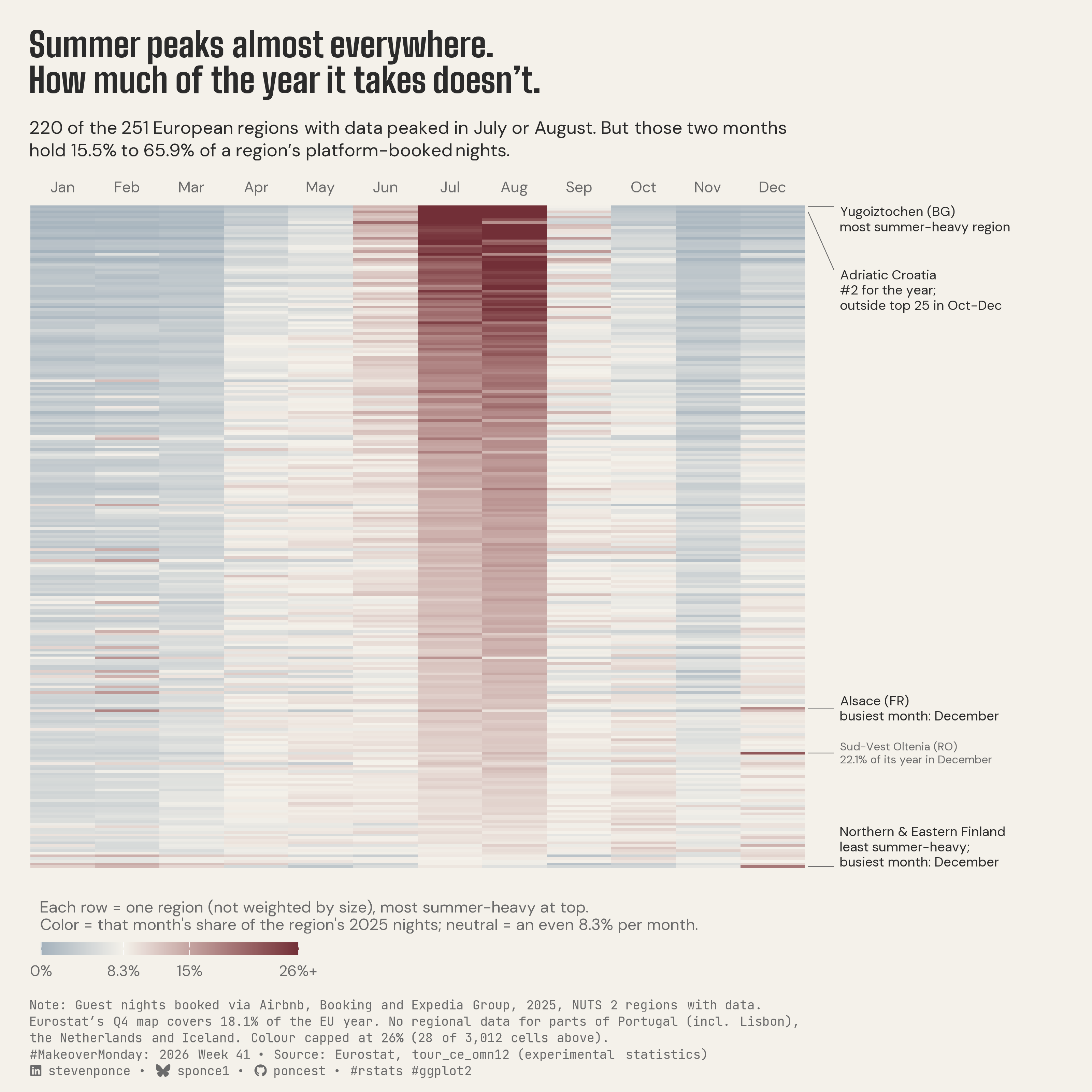
220 of the 251 European regions with data peaked in July or August. But those two months hold 15.5% to 65.9% of a region’s platform-booked nights.

MakeoverMonday
2026
A calendar heatmap of 2025 platform-booked guest nights across 251 European NUTS 2 regions shows summer peaks nearly everywhere, but July and August hold anywhere from 15.5% to 65.9% of a region’s year. Each month is shown as a share of the region’s own annual nights, so timing and concentration are compared regardless of size. Built in R with ggplot2, ggtext and ggview.
Author

Steven Ponce

Published

October 11, 2026

Original

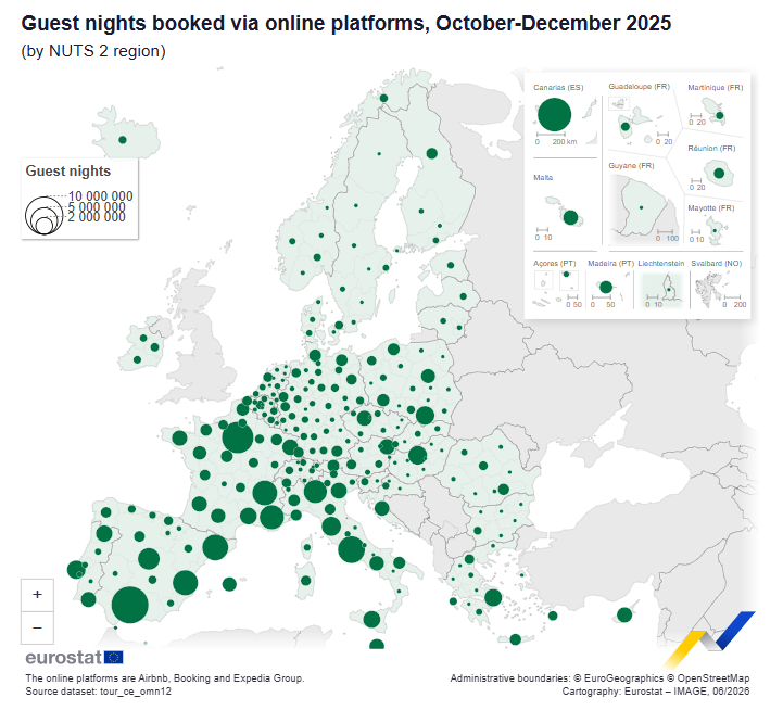
The original visualization comes from Tourism Nights Booked Through Platforms

Original visualization

Makeover

Figure 1: European NUTS 2 regions with data. Each row is one region and each column a month; color shows that month’s share of the region’s annual nights, from blue (below an even 1/12) through neutral to burgundy (26% or more). Rows run from most to least summer-heavy. A dark July–August band runs down the chart and fades toward the bottom: 220 of the 251 regions peaked in July or August, but those two months hold between 15.5% and 65.9% of a region’s nights. Yugoiztochen (Bulgaria) is the most summer-heavy region. Adriatic Croatia ranks second for the year among these regions but falls outside the top 25 in October–December. Alsace, Sud-Vest Oltenia and Northern & Eastern Finland stand out with December peaks, and Northern & Eastern Finland is the least summer-heavy. Every region gets equal space regardless of size. Regional data are missing for parts of Portugal (including Lisbon), the Netherlands, and Iceland. Source: Eurostat, tour_ce_omn12.

Steps to Create this Graphic

1. Load Packages & Setup

Show code
```{r}
#| label: load
#| warning: false
#| message: false      
#| results: "hide"     

## 1. LOAD PACKAGES & SETUP ----
suppressPackageStartupMessages({
  if (!require("pacman")) install.packages("pacman")
  pacman::p_load(
    tidyverse, ggtext, showtext, scales, glue, 
  janitor, ggview, readxl
)
})

# Source utility functions
suppressMessages(
  source(here::here("R/utils/fonts.R")))
  source(here::here("R/utils/social_icons.R"))
  source(here::here("R/themes/base_theme.R"))

### |- figure size ----
fig_w <- 10
fig_h <- 10
```

2. Read in the Data

Show code
```{r}
#| label: read
#| include: true
#| eval: true
#| warning: false
#| 

df_raw <- readxl::read_excel(
  here::here("data/MakeoverMonday/2026/Tourism_20Nights_20Booked_20Through_20Platforms_202025.xlsx"))  |>
  clean_names()

months <- c(
  "january", "february", "march", "april", "may", "june",
  "july", "august", "september", "october", "november", "december"
)
```

3. Examine the Data

Show code
```{r}
#| label: examine
#| include: true
#| eval: true
#| results: 'hide'
#| warning: false

glimpse(df_raw)
skimr::skim_without_charts(df_raw)
```

4. Tidy Data

Show code
```{r}
#| label: tidy
#| warning: false

### |- data rows: total is digits or ":" (drops Eurostat legend footer) ----
df <- df_raw |>
  filter(!is.na(geo_labels), str_detect(total, "^[0-9]+$|^:$")) |>
  select(geo = geo_labels, total, all_of(months)) |>
  mutate(across(c(total, all_of(months)), ~ as.numeric(na_if(str_trim(.x), ":"))))

### |- infer NUTS level (extract has labels only, no geo codes) ----
# Eurostat order: country -> NUTS1 -> its NUTS2 children. Integer values, so
# every NUTS1 must equal its children's sum exactly (checked below).
countries <- c(
  "Belgium", "Bulgaria", "Czechia", "Denmark", "Germany", "Estonia", "Ireland",
  "Greece", "Spain", "France", "Croatia", "Italy", "Cyprus", "Latvia",
  "Lithuania", "Luxembourg", "Hungary", "Malta", "Netherlands", "Austria",
  "Poland", "Portugal", "Romania", "Slovenia", "Slovakia", "Finland", "Sweden",
  "Iceland", "Liechtenstein", "Norway", "Switzerland"
)

infer_nuts_levels <- function(d) {
  n <- nrow(d)
  level <- rep(NA_character_, n)
  country <- rep(NA_character_, n)
  parent1 <- rep(NA_integer_, n)
  level[str_detect(d$geo, "^European Union")] <- "EU"
  level[d$geo %in% countries & d$geo != lag(d$geo, default = "")] <- "country"

  pair_start <- function(i) {
    i < n && d$geo[i + 1] == d$geo[i] &&
      identical(d$total[i + 1], d$total[i])
  }
  closes_ahead <- function(i, max_k = 20) {
    if (is.na(d$total[i])) {
      return(FALSE)
    }
    acc <- 0
    for (j in seq(i + 1, min(n, i + max_k))) {
      if (identical(level[j], "country") || is.na(d$total[j])) {
        return(FALSE)
      }
      acc <- acc + d$total[j]
      if (acc == d$total[i]) {
        return(TRUE)
      }
      if (acc > d$total[i]) {
        return(FALSE)
      }
    }
    FALSE
  }

  cur_country <- NA_character_
  cur_l1 <- NA_integer_
  remaining <- 0
  has_na <- FALSE
  for (i in seq_len(n)) {
    if (identical(level[i], "EU")) next
    if (identical(level[i], "country")) {
      cur_country <- d$geo[i]
      country[i] <- cur_country
      cur_l1 <- NA_integer_
      remaining <- 0
      has_na <- FALSE
      next
    }
    country[i] <- cur_country
    tot <- d$total[i]
    if (i > 1 && identical(level[i - 1], "nuts1") && d$geo[i - 1] == d$geo[i] &&
      identical(d$total[i - 1], tot)) {
      level[i] <- "nuts2"
      parent1[i] <- i - 1
      remaining <- 0
      has_na <- FALSE
      next
    }
    if (is.na(cur_l1) || remaining == 0 || pair_start(i) || (has_na && closes_ahead(i))) {
      level[i] <- "nuts1"
      cur_l1 <- i
      remaining <- coalesce(tot, 0)
      has_na <- FALSE
    } else {
      level[i] <- "nuts2"
      parent1[i] <- cur_l1
      if (is.na(tot)) has_na <- TRUE else remaining <- remaining - tot
    }
  }
  mutate(d, level, country, parent1)
}

geo_tbl <- infer_nuts_levels(df)

### |- hierarchy guards ----
l1_check <- geo_tbl |>
  filter(level == "nuts2") |>
  group_by(parent1) |>
  summarise(
    child_sum = sum(total, na.rm = TRUE), n_na = sum(is.na(total)),
    .groups = "drop"
  ) |>
  mutate(gap = geo_tbl$total[parent1] - child_sum)

eu_row <- geo_tbl |> filter(level == "EU")

### |- NUTS2 regions with data ----
nuts2 <- geo_tbl |>
  filter(level == "nuts2", !is.na(total)) |>
  mutate(
    julaug_share = (july + august) / total,
    q4 = october + november + december,
    q4_share = q4 / total,
    peak_month = months[max.col(across(all_of(months)), ties.method = "first")],
    rank_year = min_rank(desc(total)),
    rank_q4 = min_rank(desc(q4))
  )

cells <- nuts2 |>
  select(geo, julaug_share, total, all_of(months)) |>
  pivot_longer(all_of(months), names_to = "month", values_to = "nights") |>
  mutate(
    share = nights / total,
    month_i = match(month, months),
    row_y = as.numeric(fct_reorder(geo, julaug_share))
  ) # top = most concentrated

### |- computed facts ----
n_regions <- nrow(nuts2)
n_summer_peak <- sum(nuts2$peak_month %in% c("july", "august"))
eu_julaug <- (eu_row$july + eu_row$august) / eu_row$total
min_ja <- min(nuts2$julaug_share)
max_ja <- max(nuts2$julaug_share)
jad <- nuts2 |> filter(geo == "Jadranska Hrvatska")
eu_q4_share <- (eu_row$october + eu_row$november + eu_row$december) / eu_row$total

share_q <- quantile(cells$share, c(.99, 1))
cap <- ceiling(share_q[[1]] * 100) / 100
n_above <- sum(cells$share > cap)
pct <- \(x) paste0(format(round(100 * x, 1), nsmall = 1), "%")

### |- anchors (primary) ----
anchors <- tribble(
  ~geo, ~label, ~dy, ~vjust,
  "Yugoiztochen", "Yugoiztochen (BG)\nmost summer-heavy region", 0, 1,
  "Jadranska Hrvatska", "Adriatic Croatia\n#2 for the year;\noutside top 25 in Oct-Dec", -22, 1,
  "Alsace", "Alsace (FR)\nbusiest month: December", 0, 0.5,
  "Pohjois- ja Itä-Suomi", "Northern & Eastern Finland\nleast summer-heavy;\nbusiest month: December", 0, 0
) |>
  left_join(cells |> distinct(geo, row_y), by = "geo") |>
  mutate(label_y = row_y + dy)

### |- secondary label: darkest December row (misattribution guard) ----
show_secondary <- TRUE
dec_top <- cells |>
  filter(month == "december") |>
  slice_max(share, n = 1, with_ties = FALSE)

secondary <- tibble(
  geo = dec_top$geo, row_y = dec_top$row_y, label_y = dec_top$row_y,
  label = glue("Sud-Vest Oltenia (RO)\n{pct(dec_top$share)} of its year in December")
)
```

5. Visualization Parameters

Show code
```{r}
#| label: params
#| include: true
#| warning: false

### |-  plot aesthetics ----
colors <- get_theme_colors(
  palette = list(
    background = "#f4f1ea",
    text       = "#2b2b2b",
    muted      = "#6b6b6b"
  )
)
clrs <- colors$palette

# encoding colours as plain constants
col_high <- "#722F37"
col_low <- "#4A6F8A"
col_mid <- "#f4f1ea"

### |-  titles and caption ----
title_text <- "Summer peaks almost everywhere.<br>How much of the year it takes doesn't."

subtitle_text <- glue(
  "{n_summer_peak} of the {n_regions} European regions with data peaked in July or August. ",
  "But those two months hold {pct(min_ja)} to {pct(max_ja)} of a region's ",
  "platform-booked nights."
)

legend_title <- paste0(
  "Each row = one region (not weighted by size), most summer-heavy at top.\n",
  "Color = that month's share of the region's 2025 nights; neutral = an even 8.3% per month."
)

note_text <- glue(
  "Note: Guest nights booked via Airbnb, Booking and Expedia Group, 2025, NUTS 2 regions with data. ",
  "Eurostat's Q4 map covers {pct(eu_q4_share)} of the EU year. ",
  "No regional data for parts of Portugal (incl. Lisbon), the Netherlands and Iceland. ",
  "Colour capped at {cap * 100}% ({n_above} of {comma(nrow(cells))} cells above)."
)

caption_text <- create_mm_caption(
  mm_year = 2026,
  mm_week = 41,
  source_text = "Eurostat, tour_ce_omn12 (experimental statistics)"
)
caption_text <- glue("{note_text}<br>{caption_text}")

### |-  fonts ----
setup_fonts()
fonts <- get_font_families()
title_family <- fonts$title_1

### |-  plot theme ----
base_theme <- create_base_theme(colors)

weekly_theme <- extend_weekly_theme(
  base_theme,
  theme(
    plot.background = element_rect(fill = clrs$background, colour = NA),
    panel.background = element_rect(fill = clrs$background, colour = NA),
    panel.grid = element_blank(),
    axis.ticks = element_blank(),
    axis.text.y = element_blank(),
    axis.title = element_blank(),
    axis.text.x = element_text(size = rel(0.9), colour = clrs$muted),
    plot.title = element_textbox_simple(
      family = title_family, face = "bold", size = rel(1.6),
      lineheight = 1.05, colour = clrs$text, margin = margin(b = 14)
    ),
    plot.subtitle = element_textbox_simple(
      family = fonts$subtitle, size = rel(0.85), lineheight = 1.25,
      colour = clrs$text, margin = margin(b = 14)
    ),
    plot.caption = element_textbox_simple(
      family = fonts$caption, size = rel(0.6), lineheight = 1.3,
      colour = clrs$muted, margin = margin(t = 12)
    ),
    legend.position = "bottom",
    legend.justification = "left",
    legend.title.position = "top",
    legend.title = element_text(size = rel(0.75), colour = clrs$muted),
    legend.text = element_text(size = rel(0.7), colour = clrs$muted),
    plot.margin = margin(20, 190, 15, 20)
  )
)
theme_set(weekly_theme)
```

6. Plot

Show code
```{r}
#| label: plot
#| warning: false

### |-  main plot ----
p <- ggplot(cells, aes(month_i, row_y, fill = share)) +
  geom_tile() +
  geom_segment(
    data = anchors, aes(x = 12.55, xend = 12.95, y = row_y, yend = label_y),
    inherit.aes = FALSE, colour = clrs$muted, linewidth = 0.25
  ) +
  geom_text(
    data = anchors, aes(x = 13.05, y = label_y, label = label, vjust = vjust),
    inherit.aes = FALSE, family = fonts$text, size = 3.1, lineheight = 0.95,
    colour = clrs$text, hjust = 0
  ) +
  {
    if (show_secondary) {
      list(
        geom_segment(
          data = secondary, aes(x = 12.55, xend = 12.95, y = row_y, yend = label_y),
          inherit.aes = FALSE, colour = clrs$muted, linewidth = 0.2
        ),
        geom_text(
          data = secondary, aes(x = 13.05, y = label_y, label = label),
          inherit.aes = FALSE, family = fonts$text, size = 2.6, lineheight = 0.95,
          colour = clrs$muted, hjust = 0, vjust = 0.5
        )
      )
    }
  } +
  scale_fill_gradient2(
    low = col_low, mid = col_mid, high = col_high,
    midpoint = 1 / 12, limits = c(0, cap), oob = squish,
    breaks = c(0, 1 / 12, 0.15, cap),
    labels = c("0%", "8.3%", "15%", glue("{cap * 100}%+")),
    name = legend_title
  ) +
  scale_x_continuous(
    breaks = 1:12, labels = str_sub(str_to_title(months), 1, 3),
    expand = c(0, 0), position = "top"
  ) +
  scale_y_continuous(expand = c(0, 0)) +
  coord_cartesian(xlim = c(0.5, 12.5), clip = "off") +
  guides(fill = guide_colorbar(barwidth = unit(6, "cm"), barheight = unit(0.3, "cm"))) +
  labs(title = title_text, subtitle = subtitle_text, caption = caption_text)
```

7. Save

Show code
```{r}
#| label: save
#| warning: false

### |- save ----
main_path  <- here::here("data_visualizations", "MakeoverMonday", "2026", "mm_2026_41.png")
thumb_path <- here::here("data_visualizations", "MakeoverMonday", "2026", "thumbnails", "mm_2026_41.png")

# Full-size version, for the QMD figure
save_ggplot(
  plot = p,
  file = main_path,
  width = fig_w, height = fig_h,
  units = "in", dpi = 320,
)

# Reduced-size thumbnail
fs::dir_create(dirname(thumb_path))
magick::image_read(main_path) |>
  magick::image_resize("400") |>
  magick::image_write(thumb_path)
```

8. Session Info

TipExpand for Session Info
R version 4.6.1 (2026-06-24)
Platform: aarch64-apple-darwin23
Running under: macOS Tahoe 26.6.2

Matrix products: default
BLAS:   /Library/Frameworks/R.framework/Versions/4.6/Resources/lib/libRblas.0.dylib 
LAPACK: /Library/Frameworks/R.framework/Versions/4.6/Resources/lib/libRlapack.dylib;  LAPACK version 3.12.1

locale:
[1] en_US.UTF-8/en_US.UTF-8/en_US.UTF-8/C/en_US.UTF-8/en_US.UTF-8

time zone: America/New_York
tzcode source: internal

attached base packages:
[1] stats     graphics  grDevices utils     datasets  methods   base     

other attached packages:
 [1] here_1.0.2      readxl_1.5.0    ggview_0.2.2    janitor_2.2.1  
 [5] glue_1.8.1      scales_1.4.0    showtext_0.9-8  showtextdb_3.0 
 [9] sysfonts_0.8.9  ggtext_0.2.0    lubridate_1.9.5 forcats_1.0.1  
[13] stringr_1.6.0   dplyr_1.2.1     purrr_1.2.2     readr_2.2.0    
[17] tidyr_1.3.2     tibble_3.3.1    ggplot2_4.0.3   tidyverse_2.0.0
[21] pacman_0.5.1   

loaded via a namespace (and not attached):
 [1] gtable_0.3.6       xfun_0.60          htmlwidgets_1.6.4  tzdb_0.5.0        
 [5] vctrs_0.7.3        tools_4.6.1        generics_0.1.4     curl_7.1.0        
 [9] pkgconfig_2.0.3    RColorBrewer_1.1-3 skimr_2.2.2        S7_0.2.2          
[13] lifecycle_1.0.5    compiler_4.6.1     farver_2.1.2       textshaping_1.0.5 
[17] repr_1.1.7         codetools_0.2-20   snakecase_0.11.1   litedown_0.10     
[21] htmltools_0.5.9    yaml_2.3.12        pillar_1.11.1      magick_2.9.1      
[25] commonmark_2.0.0   tidyselect_1.2.1   digest_0.6.39      stringi_1.8.7     
[29] labeling_0.4.3     rprojroot_2.1.1    fastmap_1.2.0      grid_4.6.1        
[33] cli_3.6.6          magrittr_2.0.5     base64enc_0.1-6    withr_3.0.3       
[37] timechange_0.4.0   rmarkdown_2.31     otel_0.2.0         cellranger_1.1.0  
[41] ragg_1.5.2         hms_1.1.4          evaluate_1.0.5     knitr_1.51        
[45] markdown_2.0       rlang_1.3.0        gridtext_0.1.6     Rcpp_1.1.2        
[49] xml2_1.6.0         rstudioapi_0.19.0  jsonlite_2.0.0     R6_2.6.1          
[53] fs_2.1.0           systemfonts_1.3.2 

9. GitHub Repository

TipExpand for GitHub Repo

The complete code for this analysis is available in mm_2026_41.qmd.

For the full repository, click here.

10. References

TipExpand for References

Primary Data (Makeover Monday): 1. Makeover Monday 2026 Week 41: Tourism Nights Booked Through Platforms - XLSX: 388 rows × 27 columns (geographic label, annual total, 12 monthly columns and 13 empty flag columns), 2025 only. The extract has labels but no geographic codes, and its last 3 rows are Eurostat’s legend footer. These are Eurostat experimental statistics, built from data that Airbnb, Booking and Expedia Group share voluntarily; 2025 is the first reference year with three platforms after Tripadvisor left in late 2024. A guest night counts each person for each night, not bookings. With a single year of data, no year-over-year claim is made. - Validation of the 385 data rows: - Every annual total equals the sum of its 12 months; no monthly value is zero (the smallest is 458), and last digits are evenly spread, so there is no sign of rounding. - The EU row (951,611,862 nights) equals the sum of the 27 member-state rows exactly. - The extract reproduces the figures in Eurostat’s release: EU Q4 172.3 million; Q4 Andalucía 9.9 million, Canarias 8.2 million, Île-de-France 7.2 million, Cyprus 1,711,525; Q3 Jadranska Hrvatska 27.7 million, Andalucía 19.5 million, Provence-Alpes-Côte d’Azur 16.9 million; and a Q4 top 10 of five Spanish, three French and two Italian regions. - Geographic levels were inferred from row order (country, then each NUTS 1 region followed by its NUTS 2 regions), giving 31 country rows (EU-27 plus Iceland, Liechtenstein, Norway and Switzerland), 96 NUTS 1 rows and 257 NUTS 2 rows. Because the values are whole numbers, every NUTS 1 region whose NUTS 2 regions all have data must equal their sum exactly, and all of them do. Labels repeat across levels for single-region units (e.g., Brussels, Berlin, Cyprus, Malta, Luxembourg). - Coverage gaps: - Seven rows are entirely unavailable: five regions from the retired NUTS 2021 classification (Utrecht, Zuid-Holland, Centro (PT), Área Metropolitana de Lisboa, Alentejo) and Iceland’s two regional rows. Their replacement regions are not in this extract. - Nights with no NUTS 2 region in the extract: Portugal 18,251,104 (36.9%, including Lisbon), the Netherlands 2,062,354 (17.3%) and Iceland 2,708,531 (100%). - Nights not assigned to any region: Switzerland 65,100 (0.6%) and Greece 2,006. These affect no claim in the chart. - The analysis uses the 251 NUTS 2 regions with data, and every regional count is stated as “with data”. - The original is Eurostat’s map of October–December 2025 guest nights by NUTS 2 region, with circle area showing absolute nights. That quarter holds 18.1% of the EU’s annual nights, and large circles partly reflect large regions. Across all regions, the Q4 ranking stays close to the annual one (Spearman 0.959; 9 of the top 10 shared). The regions that drop are the most summer-concentrated: Jadranska Hrvatska is 2nd for the year but 27th in Q4 among regions with data, with 4.1% of its nights in October–December; Ionia Nisia falls from 28th to 92nd and Notio Aigaio from 24th to 68th. Missing regions can only push these Q4 ranks lower, so the chart states “outside the top 25” rather than an exact rank. - This makeover changes the question from how many nights a region has to when they occur. Each cell is that month’s share of the region’s annual nights, and each region gets one row of equal height regardless of size, ordered by its July–August share. Colour diverges around an even month (1/12) and is capped at 26%, just above the 99th percentile of monthly shares; 28 of the 3,012 cells exceed the cap. - Key figures: - Summer peaks: 220 of 251 regions (87.6%) had their busiest month in July or August. This counts regions, not nights. - Concentration: July and August hold between 15.5% (Pohjois- ja Itä-Suomi) and 65.9% (Yugoiztochen) of a region’s annual nights, with a median of 28.8%; two months are 16.7% of a calendar year. For the EU as a whole, weighted by nights, the share is 33.1%. - Peaks outside summer: 30 regions peak outside June–September, but 9 of them lead their second-busiest month by less than 5% (Comunidad de Madrid’s October leads May by 1.1%), so none of these is labelled. The labelled December peaks are clear: Alsace leads its second-busiest month by 34%, Pohjois- ja Itä-Suomi by 43%, and Sud-Vest Oltenia by 66%. Sud-Vest Oltenia has the largest December share of any region (22.1%) despite only about 257,000 annual nights, which shows why equal rows are disclosed. Six of the ten regions that peak in October are German. No cause is claimed for any of these peaks. - One signal, not two: July–August share and Q4 share correlate at ρ = −0.90. Because both are fractions of the same annual total, part of that relationship is built in, so they are treated as a single seasonal measure.

Source Data: 2. Eurostat, Nights spent at short-term rental accommodation booked via online platforms (tour_ce_omn12), custom extract, monthly 2025, by NUTS 2 region (accessed October 2026) 3. Eurostat news, 2 July 2026, Short-term rental nights booked via online platforms

11. Custom Functions Documentation

Note📦 Custom Helper Functions

This analysis uses custom functions from my personal module library for efficiency and consistency across projects.

Functions Used:

  • fonts.R: setup_fonts(), get_font_families() - Font management with showtext
  • social_icons.R: create_social_caption() - Generates formatted social media captions
  • image_utils.R: save_plot() - Consistent plot saving with naming conventions
  • base_theme.R: create_base_theme(), extend_weekly_theme(), get_theme_colors() - Custom ggplot2 themes

Why custom functions?
These utilities standardize theming, fonts, and output across all my data visualizations. The core analysis (data tidying and visualization logic) uses only standard tidyverse packages.

Source Code:
View all custom functions → GitHub: R/utils

Back to top

Citation

BibTeX citation:
@online{ponce2026,
  author = {Ponce, Steven},
  title = {Summer Peaks Almost Everywhere. {How} Much of the Year It
    Takes Doesn’t.},
  date = {2026-10-11},
  url = {https://stevenponce.netlify.app/data_visualizations/MakeoverMonday/2026/mm_2026_41.html},
  langid = {en}
}
For attribution, please cite this work as:
Ponce, Steven. 2026. “Summer Peaks Almost Everywhere. How Much of the Year It Takes Doesn’t.” October 11. https://stevenponce.netlify.app/data_visualizations/MakeoverMonday/2026/mm_2026_41.html.
Source Code
---
title: "Summer peaks almost everywhere. How much of the year it takes doesn't."
subtitle: "220 of the 251 European regions with data peaked in July or August. But those two months hold 15.5% to 65.9% of a region's platform-booked nights."
description: "A calendar heatmap of 2025 platform-booked guest nights across 251 European NUTS 2 regions shows summer peaks nearly everywhere, but July and August hold anywhere from 15.5% to 65.9% of a region's year. Each month is shown as a share of the region's own annual nights, so timing and concentration are compared regardless of size. Built in R with ggplot2, ggtext and ggview."
date: "2026-10-11"
author:
  - name: "Steven Ponce"
    url: "https://stevenponce.netlify.app"
citation:
  url: "https://stevenponce.netlify.app/data_visualizations/MakeoverMonday/2026/mm_2026_41.html"
categories: ["MakeoverMonday", "2026"]
tags: [
  "makeover-monday",
  "heatmap",
  "calendar-heatmap",
  "seasonality",
  "tourism",
  "short-term-rentals",
  "eurostat",
  "nuts-2",
  "europe",
  "annotation",
  "ggplot2",
  "ggtext",
  "ggview",
  "2026"
]
image: "thumbnails/mm_2026_41.png"
format:
  html:
    toc: true
    toc-depth: 5
    code-link: true
    code-fold: true
    code-tools: true
    code-summary: "Show code"
editor_options: 
  chunk_output_type: inline
execute: 
  freeze: true
  cache: true
  error: false
  message: false
  warning: false
  eval: true
---

```{r}
#| label: setup-links
#| include: false

# CENTRALIZED LINK MANAGEMENT

## Project-specific info 
current_year <- 2026
current_week <- 41
project_file <- "mm_2026_41.qmd"
project_image <- "mm_2026_41.png"

## Data Sources
data_main <- "https://ec.europa.eu/eurostat/web/products-eurostat-news/w/ddn-20260702-1"
data_secondary <- "https://ec.europa.eu/eurostat/databrowser/view/tour_ce_omn12__custom_15997748/bookmark/table?lang=en&bookmarkId=3cebcd02-17c5-4393-be50-dcd8d670f4ac&c=1742994015070"

## Repository Links  
repo_main <- "https://github.com/poncest/personal-website/"
repo_file <- paste0("https://github.com/poncest/personal-website/blob/master/data_visualizations/MakeoverMonday/", current_year, "/", project_file)

## External Resources/Images
chart_original <- "https://raw.githubusercontent.com/poncest/MakeoverMonday/refs/heads/master/2026/Week_41/original_chart.png"

## Organization/Platform Links
org_primary <- "https://ec.europa.eu/eurostat/web/products-eurostat-news/w/ddn-20260702-1"
org_secondary <- "https://ec.europa.eu/eurostat/web/products-eurostat-news/w/ddn-20260702-1"

# Helper function to create markdown links
create_link <- function(text, url) {
  paste0("[", text, "](", url, ")")
}

# Helper function for citation-style links
create_citation_link <- function(text, url, title = NULL) {
  if (is.null(title)) {
    paste0("[", text, "](", url, ")")
  } else {
    paste0("[", text, "](", url, ' "', title, '")')
  }
}
```

### Original

The original visualization comes from `r create_link("Tourism Nights Booked Through Platforms", org_primary)`
![Original visualization](https://raw.githubusercontent.com/poncest/MakeoverMonday/refs/heads/master/2026/Week_41/original_chart.png)

### Makeover

![European NUTS 2 regions with data. Each row is one region and each column a month; color shows that month's share of the region's annual nights, from blue (below an even 1/12) through neutral to burgundy (26% or more). Rows run from most to least summer-heavy. A dark July–August band runs down the chart and fades toward the bottom: 220 of the 251 regions peaked in July or August, but those two months hold between 15.5% and 65.9% of a region's nights. Yugoiztochen (Bulgaria) is the most summer-heavy region. Adriatic Croatia ranks second for the year among these regions but falls outside the top 25 in October–December. Alsace, Sud-Vest Oltenia and Northern & Eastern Finland stand out with December peaks, and Northern & Eastern Finland is the least summer-heavy. Every region gets equal space regardless of size. Regional data are missing for parts of Portugal (including Lisbon), the Netherlands, and Iceland. Source: Eurostat, tour_ce_omn12.](mm_2026_41.png){#fig-1}

### [**Steps to Create this Graphic**]{.mark}

#### [1. Load Packages & Setup]{.smallcaps}

```{r}
#| label: load
#| warning: false
#| message: false      
#| results: "hide"     

## 1. LOAD PACKAGES & SETUP ----
suppressPackageStartupMessages({
  if (!require("pacman")) install.packages("pacman")
  pacman::p_load(
    tidyverse, ggtext, showtext, scales, glue, 
  janitor, ggview, readxl
)
})

# Source utility functions
suppressMessages(
  source(here::here("R/utils/fonts.R")))
  source(here::here("R/utils/social_icons.R"))
  source(here::here("R/themes/base_theme.R"))

### |- figure size ----
fig_w <- 10
fig_h <- 10
```

#### [2. Read in the Data]{.smallcaps}

```{r}
#| label: read
#| include: true
#| eval: true
#| warning: false
#| 

df_raw <- readxl::read_excel(
  here::here("data/MakeoverMonday/2026/Tourism_20Nights_20Booked_20Through_20Platforms_202025.xlsx"))  |>
  clean_names()

months <- c(
  "january", "february", "march", "april", "may", "june",
  "july", "august", "september", "october", "november", "december"
)
```

#### [3. Examine the Data]{.smallcaps}

```{r}
#| label: examine
#| include: true
#| eval: true
#| results: 'hide'
#| warning: false

glimpse(df_raw)
skimr::skim_without_charts(df_raw)
```

#### [4. Tidy Data]{.smallcaps}

```{r}
#| label: tidy
#| warning: false

### |- data rows: total is digits or ":" (drops Eurostat legend footer) ----
df <- df_raw |>
  filter(!is.na(geo_labels), str_detect(total, "^[0-9]+$|^:$")) |>
  select(geo = geo_labels, total, all_of(months)) |>
  mutate(across(c(total, all_of(months)), ~ as.numeric(na_if(str_trim(.x), ":"))))

### |- infer NUTS level (extract has labels only, no geo codes) ----
# Eurostat order: country -> NUTS1 -> its NUTS2 children. Integer values, so
# every NUTS1 must equal its children's sum exactly (checked below).
countries <- c(
  "Belgium", "Bulgaria", "Czechia", "Denmark", "Germany", "Estonia", "Ireland",
  "Greece", "Spain", "France", "Croatia", "Italy", "Cyprus", "Latvia",
  "Lithuania", "Luxembourg", "Hungary", "Malta", "Netherlands", "Austria",
  "Poland", "Portugal", "Romania", "Slovenia", "Slovakia", "Finland", "Sweden",
  "Iceland", "Liechtenstein", "Norway", "Switzerland"
)

infer_nuts_levels <- function(d) {
  n <- nrow(d)
  level <- rep(NA_character_, n)
  country <- rep(NA_character_, n)
  parent1 <- rep(NA_integer_, n)
  level[str_detect(d$geo, "^European Union")] <- "EU"
  level[d$geo %in% countries & d$geo != lag(d$geo, default = "")] <- "country"

  pair_start <- function(i) {
    i < n && d$geo[i + 1] == d$geo[i] &&
      identical(d$total[i + 1], d$total[i])
  }
  closes_ahead <- function(i, max_k = 20) {
    if (is.na(d$total[i])) {
      return(FALSE)
    }
    acc <- 0
    for (j in seq(i + 1, min(n, i + max_k))) {
      if (identical(level[j], "country") || is.na(d$total[j])) {
        return(FALSE)
      }
      acc <- acc + d$total[j]
      if (acc == d$total[i]) {
        return(TRUE)
      }
      if (acc > d$total[i]) {
        return(FALSE)
      }
    }
    FALSE
  }

  cur_country <- NA_character_
  cur_l1 <- NA_integer_
  remaining <- 0
  has_na <- FALSE
  for (i in seq_len(n)) {
    if (identical(level[i], "EU")) next
    if (identical(level[i], "country")) {
      cur_country <- d$geo[i]
      country[i] <- cur_country
      cur_l1 <- NA_integer_
      remaining <- 0
      has_na <- FALSE
      next
    }
    country[i] <- cur_country
    tot <- d$total[i]
    if (i > 1 && identical(level[i - 1], "nuts1") && d$geo[i - 1] == d$geo[i] &&
      identical(d$total[i - 1], tot)) {
      level[i] <- "nuts2"
      parent1[i] <- i - 1
      remaining <- 0
      has_na <- FALSE
      next
    }
    if (is.na(cur_l1) || remaining == 0 || pair_start(i) || (has_na && closes_ahead(i))) {
      level[i] <- "nuts1"
      cur_l1 <- i
      remaining <- coalesce(tot, 0)
      has_na <- FALSE
    } else {
      level[i] <- "nuts2"
      parent1[i] <- cur_l1
      if (is.na(tot)) has_na <- TRUE else remaining <- remaining - tot
    }
  }
  mutate(d, level, country, parent1)
}

geo_tbl <- infer_nuts_levels(df)

### |- hierarchy guards ----
l1_check <- geo_tbl |>
  filter(level == "nuts2") |>
  group_by(parent1) |>
  summarise(
    child_sum = sum(total, na.rm = TRUE), n_na = sum(is.na(total)),
    .groups = "drop"
  ) |>
  mutate(gap = geo_tbl$total[parent1] - child_sum)

eu_row <- geo_tbl |> filter(level == "EU")

### |- NUTS2 regions with data ----
nuts2 <- geo_tbl |>
  filter(level == "nuts2", !is.na(total)) |>
  mutate(
    julaug_share = (july + august) / total,
    q4 = october + november + december,
    q4_share = q4 / total,
    peak_month = months[max.col(across(all_of(months)), ties.method = "first")],
    rank_year = min_rank(desc(total)),
    rank_q4 = min_rank(desc(q4))
  )

cells <- nuts2 |>
  select(geo, julaug_share, total, all_of(months)) |>
  pivot_longer(all_of(months), names_to = "month", values_to = "nights") |>
  mutate(
    share = nights / total,
    month_i = match(month, months),
    row_y = as.numeric(fct_reorder(geo, julaug_share))
  ) # top = most concentrated

### |- computed facts ----
n_regions <- nrow(nuts2)
n_summer_peak <- sum(nuts2$peak_month %in% c("july", "august"))
eu_julaug <- (eu_row$july + eu_row$august) / eu_row$total
min_ja <- min(nuts2$julaug_share)
max_ja <- max(nuts2$julaug_share)
jad <- nuts2 |> filter(geo == "Jadranska Hrvatska")
eu_q4_share <- (eu_row$october + eu_row$november + eu_row$december) / eu_row$total

share_q <- quantile(cells$share, c(.99, 1))
cap <- ceiling(share_q[[1]] * 100) / 100
n_above <- sum(cells$share > cap)
pct <- \(x) paste0(format(round(100 * x, 1), nsmall = 1), "%")

### |- anchors (primary) ----
anchors <- tribble(
  ~geo, ~label, ~dy, ~vjust,
  "Yugoiztochen", "Yugoiztochen (BG)\nmost summer-heavy region", 0, 1,
  "Jadranska Hrvatska", "Adriatic Croatia\n#2 for the year;\noutside top 25 in Oct-Dec", -22, 1,
  "Alsace", "Alsace (FR)\nbusiest month: December", 0, 0.5,
  "Pohjois- ja Itä-Suomi", "Northern & Eastern Finland\nleast summer-heavy;\nbusiest month: December", 0, 0
) |>
  left_join(cells |> distinct(geo, row_y), by = "geo") |>
  mutate(label_y = row_y + dy)

### |- secondary label: darkest December row (misattribution guard) ----
show_secondary <- TRUE
dec_top <- cells |>
  filter(month == "december") |>
  slice_max(share, n = 1, with_ties = FALSE)

secondary <- tibble(
  geo = dec_top$geo, row_y = dec_top$row_y, label_y = dec_top$row_y,
  label = glue("Sud-Vest Oltenia (RO)\n{pct(dec_top$share)} of its year in December")
)
```

#### [5. Visualization Parameters]{.smallcaps}

```{r}
#| label: params
#| include: true
#| warning: false

### |-  plot aesthetics ----
colors <- get_theme_colors(
  palette = list(
    background = "#f4f1ea",
    text       = "#2b2b2b",
    muted      = "#6b6b6b"
  )
)
clrs <- colors$palette

# encoding colours as plain constants
col_high <- "#722F37"
col_low <- "#4A6F8A"
col_mid <- "#f4f1ea"

### |-  titles and caption ----
title_text <- "Summer peaks almost everywhere.<br>How much of the year it takes doesn't."

subtitle_text <- glue(
  "{n_summer_peak} of the {n_regions} European regions with data peaked in July or August. ",
  "But those two months hold {pct(min_ja)} to {pct(max_ja)} of a region's ",
  "platform-booked nights."
)

legend_title <- paste0(
  "Each row = one region (not weighted by size), most summer-heavy at top.\n",
  "Color = that month's share of the region's 2025 nights; neutral = an even 8.3% per month."
)

note_text <- glue(
  "Note: Guest nights booked via Airbnb, Booking and Expedia Group, 2025, NUTS 2 regions with data. ",
  "Eurostat's Q4 map covers {pct(eu_q4_share)} of the EU year. ",
  "No regional data for parts of Portugal (incl. Lisbon), the Netherlands and Iceland. ",
  "Colour capped at {cap * 100}% ({n_above} of {comma(nrow(cells))} cells above)."
)

caption_text <- create_mm_caption(
  mm_year = 2026,
  mm_week = 41,
  source_text = "Eurostat, tour_ce_omn12 (experimental statistics)"
)
caption_text <- glue("{note_text}<br>{caption_text}")

### |-  fonts ----
setup_fonts()
fonts <- get_font_families()
title_family <- fonts$title_1

### |-  plot theme ----
base_theme <- create_base_theme(colors)

weekly_theme <- extend_weekly_theme(
  base_theme,
  theme(
    plot.background = element_rect(fill = clrs$background, colour = NA),
    panel.background = element_rect(fill = clrs$background, colour = NA),
    panel.grid = element_blank(),
    axis.ticks = element_blank(),
    axis.text.y = element_blank(),
    axis.title = element_blank(),
    axis.text.x = element_text(size = rel(0.9), colour = clrs$muted),
    plot.title = element_textbox_simple(
      family = title_family, face = "bold", size = rel(1.6),
      lineheight = 1.05, colour = clrs$text, margin = margin(b = 14)
    ),
    plot.subtitle = element_textbox_simple(
      family = fonts$subtitle, size = rel(0.85), lineheight = 1.25,
      colour = clrs$text, margin = margin(b = 14)
    ),
    plot.caption = element_textbox_simple(
      family = fonts$caption, size = rel(0.6), lineheight = 1.3,
      colour = clrs$muted, margin = margin(t = 12)
    ),
    legend.position = "bottom",
    legend.justification = "left",
    legend.title.position = "top",
    legend.title = element_text(size = rel(0.75), colour = clrs$muted),
    legend.text = element_text(size = rel(0.7), colour = clrs$muted),
    plot.margin = margin(20, 190, 15, 20)
  )
)
theme_set(weekly_theme)
```

#### [6. Plot]{.smallcaps}

```{r}
#| label: plot
#| warning: false

### |-  main plot ----
p <- ggplot(cells, aes(month_i, row_y, fill = share)) +
  geom_tile() +
  geom_segment(
    data = anchors, aes(x = 12.55, xend = 12.95, y = row_y, yend = label_y),
    inherit.aes = FALSE, colour = clrs$muted, linewidth = 0.25
  ) +
  geom_text(
    data = anchors, aes(x = 13.05, y = label_y, label = label, vjust = vjust),
    inherit.aes = FALSE, family = fonts$text, size = 3.1, lineheight = 0.95,
    colour = clrs$text, hjust = 0
  ) +
  {
    if (show_secondary) {
      list(
        geom_segment(
          data = secondary, aes(x = 12.55, xend = 12.95, y = row_y, yend = label_y),
          inherit.aes = FALSE, colour = clrs$muted, linewidth = 0.2
        ),
        geom_text(
          data = secondary, aes(x = 13.05, y = label_y, label = label),
          inherit.aes = FALSE, family = fonts$text, size = 2.6, lineheight = 0.95,
          colour = clrs$muted, hjust = 0, vjust = 0.5
        )
      )
    }
  } +
  scale_fill_gradient2(
    low = col_low, mid = col_mid, high = col_high,
    midpoint = 1 / 12, limits = c(0, cap), oob = squish,
    breaks = c(0, 1 / 12, 0.15, cap),
    labels = c("0%", "8.3%", "15%", glue("{cap * 100}%+")),
    name = legend_title
  ) +
  scale_x_continuous(
    breaks = 1:12, labels = str_sub(str_to_title(months), 1, 3),
    expand = c(0, 0), position = "top"
  ) +
  scale_y_continuous(expand = c(0, 0)) +
  coord_cartesian(xlim = c(0.5, 12.5), clip = "off") +
  guides(fill = guide_colorbar(barwidth = unit(6, "cm"), barheight = unit(0.3, "cm"))) +
  labs(title = title_text, subtitle = subtitle_text, caption = caption_text)
```

#### [7. Save]{.smallcaps}

```{r}
#| label: save
#| warning: false

### |- save ----
main_path  <- here::here("data_visualizations", "MakeoverMonday", "2026", "mm_2026_41.png")
thumb_path <- here::here("data_visualizations", "MakeoverMonday", "2026", "thumbnails", "mm_2026_41.png")

# Full-size version, for the QMD figure
save_ggplot(
  plot = p,
  file = main_path,
  width = fig_w, height = fig_h,
  units = "in", dpi = 320,
)

# Reduced-size thumbnail
fs::dir_create(dirname(thumb_path))
magick::image_read(main_path) |>
  magick::image_resize("400") |>
  magick::image_write(thumb_path)
```

#### [8. Session Info]{.smallcaps}

::: {.callout-tip collapse="true"}
##### Expand for Session Info

```{r, echo = FALSE}
#| eval: true
#| warning: false

sessionInfo()
```
:::

#### [9. GitHub Repository]{.smallcaps}

::: {.callout-tip collapse="true"}
##### Expand for GitHub Repo

The complete code for this analysis is available in `r create_link(project_file, repo_file)`.

For the full repository, `r create_link("click here", repo_main)`.
:::

#### [10. References]{.smallcaps}
::: {.callout-tip collapse="true"}
##### Expand for References

**Primary Data (Makeover Monday):**
1. Makeover Monday 2026 Week 41: `r create_link("Tourism Nights Booked Through Platforms", "https://ec.europa.eu/eurostat/web/products-eurostat-news/w/ddn-20260702-1")`
   - XLSX: 388 rows × 27 columns (geographic label, annual total, 12 monthly columns and 13 empty flag columns), 2025 only. The extract has labels but no geographic codes, and its last 3 rows are Eurostat's legend footer. These are Eurostat experimental statistics, built from data that Airbnb, Booking and Expedia Group share voluntarily; 2025 is the first reference year with three platforms after Tripadvisor left in late 2024. A guest night counts each person for each night, not bookings. With a single year of data, no year-over-year claim is made.
   - Validation of the 385 data rows:
     - Every annual total equals the sum of its 12 months; no monthly value is zero (the smallest is 458), and last digits are evenly spread, so there is no sign of rounding.
     - The EU row (951,611,862 nights) equals the sum of the 27 member-state rows exactly.
     - The extract reproduces the figures in Eurostat's release: EU Q4 172.3 million; Q4 Andalucía 9.9 million, Canarias 8.2 million, Île-de-France 7.2 million, Cyprus 1,711,525; Q3 Jadranska Hrvatska 27.7 million, Andalucía 19.5 million, Provence-Alpes-Côte d'Azur 16.9 million; and a Q4 top 10 of five Spanish, three French and two Italian regions.
   - Geographic levels were inferred from row order (country, then each NUTS 1 region followed by its NUTS 2 regions), giving 31 country rows (EU-27 plus Iceland, Liechtenstein, Norway and Switzerland), 96 NUTS 1 rows and 257 NUTS 2 rows. Because the values are whole numbers, every NUTS 1 region whose NUTS 2 regions all have data must equal their sum exactly, and all of them do. Labels repeat across levels for single-region units (e.g., Brussels, Berlin, Cyprus, Malta, Luxembourg).
   - Coverage gaps:
     - Seven rows are entirely unavailable: five regions from the retired NUTS 2021 classification (Utrecht, Zuid-Holland, Centro (PT), Área Metropolitana de Lisboa, Alentejo) and Iceland's two regional rows. Their replacement regions are not in this extract.
     - Nights with no NUTS 2 region in the extract: Portugal 18,251,104 (36.9%, including Lisbon), the Netherlands 2,062,354 (17.3%) and Iceland 2,708,531 (100%).
     - Nights not assigned to any region: Switzerland 65,100 (0.6%) and Greece 2,006. These affect no claim in the chart.
     - The analysis uses the 251 NUTS 2 regions with data, and every regional count is stated as "with data".
   - The original is Eurostat's map of October–December 2025 guest nights by NUTS 2 region, with circle area showing absolute nights. That quarter holds 18.1% of the EU's annual nights, and large circles partly reflect large regions. Across all regions, the Q4 ranking stays close to the annual one (Spearman 0.959; 9 of the top 10 shared). The regions that drop are the most summer-concentrated: Jadranska Hrvatska is 2nd for the year but 27th in Q4 among regions with data, with 4.1% of its nights in October–December; Ionia Nisia falls from 28th to 92nd and Notio Aigaio from 24th to 68th. Missing regions can only push these Q4 ranks lower, so the chart states "outside the top 25" rather than an exact rank.
   - This makeover changes the question from how many nights a region has to when they occur. Each cell is that month's share of the region's annual nights, and each region gets one row of equal height regardless of size, ordered by its July–August share. Colour diverges around an even month (1/12) and is capped at 26%, just above the 99th percentile of monthly shares; 28 of the 3,012 cells exceed the cap.
   - Key figures:
     - **Summer peaks:** 220 of 251 regions (87.6%) had their busiest month in July or August. This counts regions, not nights.
     - **Concentration:** July and August hold between 15.5% (Pohjois- ja Itä-Suomi) and 65.9% (Yugoiztochen) of a region's annual nights, with a median of 28.8%; two months are 16.7% of a calendar year. For the EU as a whole, weighted by nights, the share is 33.1%.
     - **Peaks outside summer:** 30 regions peak outside June–September, but 9 of them lead their second-busiest month by less than 5% (Comunidad de Madrid's October leads May by 1.1%), so none of these is labelled. The labelled December peaks are clear: Alsace leads its second-busiest month by 34%, Pohjois- ja Itä-Suomi by 43%, and Sud-Vest Oltenia by 66%. Sud-Vest Oltenia has the largest December share of any region (22.1%) despite only about 257,000 annual nights, which shows why equal rows are disclosed. Six of the ten regions that peak in October are German. No cause is claimed for any of these peaks.
     - **One signal, not two:** July–August share and Q4 share correlate at ρ = −0.90. Because both are fractions of the same annual total, part of that relationship is built in, so they are treated as a single seasonal measure.

**Source Data:**
2. Eurostat, `r create_link("Nights spent at short-term rental accommodation booked via online platforms (tour_ce_omn12)", "https://ec.europa.eu/eurostat/databrowser/view/tour_ce_omn12__custom_15997748/bookmark/table?lang=en&bookmarkId=3cebcd02-17c5-4393-be50-dcd8d670f4ac&c=1742994015070")`, custom extract, monthly 2025, by NUTS 2 region (accessed October 2026)
3. Eurostat news, 2 July 2026, `r create_link("Short-term rental nights booked via online platforms", "https://ec.europa.eu/eurostat/web/products-eurostat-news/w/ddn-20260702-1")`
:::


#### [11. Custom Functions Documentation]{.smallcaps}

::: {.callout-note collapse="true"}
##### 📦 Custom Helper Functions

This analysis uses custom functions from my personal module library for efficiency and consistency across projects.

**Functions Used:**

-   **`fonts.R`**: `setup_fonts()`, `get_font_families()` - Font management with showtext
-   **`social_icons.R`**: `create_social_caption()` - Generates formatted social media captions
-   **`image_utils.R`**: `save_plot()` - Consistent plot saving with naming conventions
-   **`base_theme.R`**: `create_base_theme()`, `extend_weekly_theme()`, `get_theme_colors()` - Custom ggplot2 themes

**Why custom functions?**\
These utilities standardize theming, fonts, and output across all my data visualizations. The core analysis (data tidying and visualization logic) uses only standard tidyverse packages.

**Source Code:**\
View all custom functions → [GitHub: R/utils](https://github.com/poncest/personal-website/tree/master/R)
:::

© 2026 Steven Ponce · Built with R + Quarto

Source Issues
