---
title: "The original thirteen didn't fade equally"
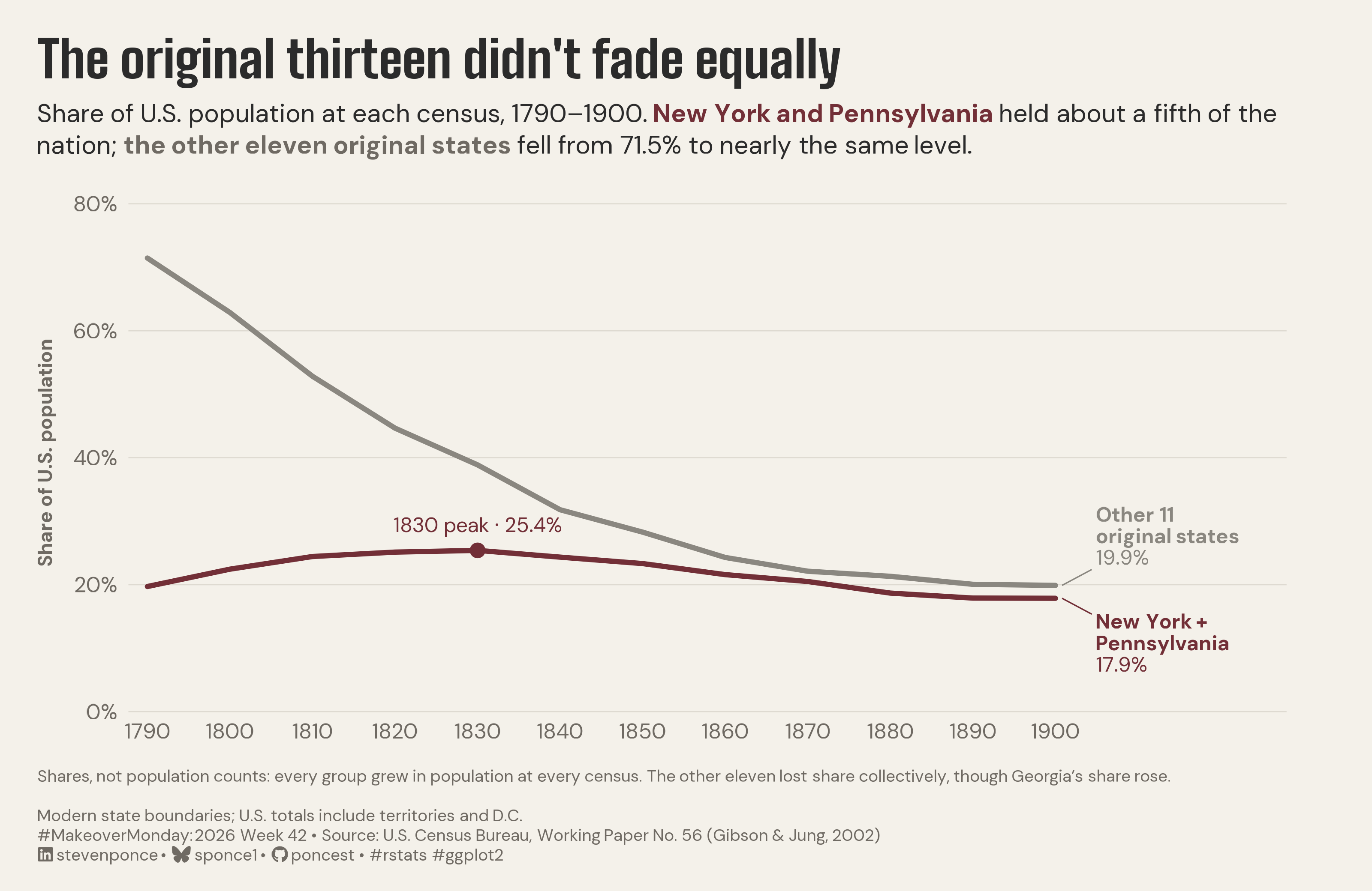
subtitle: "Share of U.S. population at each census, 1790–1900. New York and Pennsylvania held about a fifth of the nation; the other eleven original states fell from 71.5% to nearly the same level."
description: "A two-line chart of national population share, 1790–1900, shows New York and Pennsylvania holding about a fifth of the U.S. while the other eleven original states fell from 71.5% to 19.9%. Grouped shares on modern state boundaries recast the 1883 atlas's rank chart as magnitude. Built in R with ggplot2, ggtext, and showtext."
date: "2026-10-18"
author:
- name: "Steven Ponce"
url: "https://stevenponce.netlify.app"
citation:
url: "https://stevenponce.netlify.app/data_visualizations/MakeoverMonday/2026/mm_2026_42.html"
categories: ["MakeoverMonday", "2026"]
tags: [
"makeover-monday",
"data-visualization",
"ggplot2",
"line-chart",
"census",
"us-history",
"population",
"population-share",
"historical-data",
"original-thirteen",
"ggtext",
"direct-labeling",
"2026"
]
image: "thumbnails/mm_2026_42.png"
format:
html:
toc: true
toc-depth: 5
code-link: true
code-fold: true
code-tools: true
code-summary: "Show code"
editor_options:
chunk_output_type: inline
execute:
freeze: true
cache: true
error: false
message: false
warning: false
eval: true
---
```{r}
#| label: setup-links
#| include: false
# CENTRALIZED LINK MANAGEMENT
## Project-specific info
current_year <- 2026
current_week <- 42
project_file <- "mm_2026_42.qmd"
project_image <- "mm_2026_42.png"
## Data Sources
data_main <- "https://www.census.gov/library/working-papers/2002/demo/POP-twps0056.html"
data_secondary <- "https://www.census.gov/library/working-papers/2002/demo/POP-twps0056.html"
## Repository Links
repo_main <- "https://github.com/poncest/personal-website/"
repo_file <- paste0("https://github.com/poncest/personal-website/blob/master/data_visualizations/MakeoverMonday/", current_year, "/", project_file)
## External Resources/Images
chart_original <- "https://raw.githubusercontent.com/poncest/MakeoverMonday/refs/heads/master/2026/Week_42/original_chart.png"
## Organization/Platform Links
org_primary <- "https://blogs.loc.gov/maps/2022/12/gannett-and-hewes-visualizations-of-the-1880-census/"
org_secondary <- "https://blogs.loc.gov/maps/2022/12/gannett-and-hewes-visualizations-of-the-1880-census/"
# Helper function to create markdown links
create_link <- function(text, url) {
paste0("[", text, "](", url, ")")
}
# Helper function for citation-style links
create_citation_link <- function(text, url, title = NULL) {
if (is.null(title)) {
paste0("[", text, "](", url, ")")
} else {
paste0("[", text, "](", url, ' "', title, '")')
}
}
```
### Original
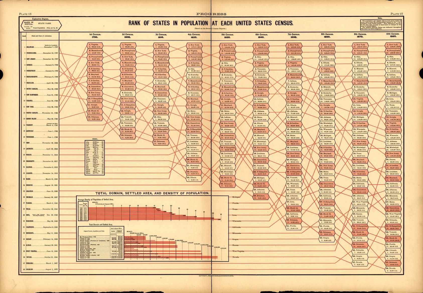
The original visualization comes from `r create_link("The First Century of the U.S. Census", org_primary)`
### Makeover
{#fig-1}
### [**Steps to Create this Graphic**]{.mark}
#### [1. Load Packages & Setup]{.smallcaps}
```{r}
#| label: load
#| warning: false
#| message: false
#| results: "hide"

## 1. LOAD PACKAGES & SETUP ----
suppressPackageStartupMessages({
  if (!require("pacman")) install.packages("pacman")
  pacman::p_load(
    tidyverse, ggtext, showtext, scales, glue,
  janitor, ggview, readxl
)
})

# Source utility functions
suppressMessages(
  source(here::here("R/utils/fonts.R")))
  source(here::here("R/utils/social_icons.R"))
  source(here::here("R/themes/base_theme.R"))

### |- figure size ----
fig_w <- 10
fig_h <- 6.5
fig_dpi <- 320

### |-  fonts ----
setup_fonts()
fonts <- get_font_families()
title_family <- fonts$title_1
text_family  <- fonts$text
```
#### [2. Read in the Data]{.smallcaps}
```{r}
#| label: read
#| include: true
#| eval: true
#| warning: false
#|

df_raw <- read_csv(
  here::here("data/MakeoverMonday/2026/us_state_population_1790_1990.csv"),
  col_types = cols(.default = col_character()),
  na = character()
) |>
  clean_names() |>
  mutate(
    year = as.integer(year),
    population = as.numeric(population)
  )
```
#### [3. Examine the Data]{.smallcaps}
```{r}
#| label: examine
#| include: true
#| eval: true
#| results: 'hide'
#| warning: false

glimpse(df_raw)
skimr::skim_without_charts(df_raw)
```
#### [4. Tidy Data]{.smallcaps}
```{r}
#| label: tidy
#| warning: false

two_states <- c("New York", "Pennsylvania")
original_13 <- c(
  "Connecticut", "Delaware", "Georgia", "Maryland", "Massachusetts",
  "New Hampshire", "New Jersey", "New York", "North Carolina",
  "Pennsylvania", "Rhode Island", "South Carolina", "Virginia"
)
grp_two <- "New York + Pennsylvania"
grp_eleven <- "Other 11 original states"

shares <- df_raw |>
  filter(year <= 1900) |>
  mutate(group = case_when(
    state %in% two_states ~ grp_two,
    state %in% original_13 ~ grp_eleven,
    .default = "Rest of U.S."
  )) |>
  summarise(pop = sum(population), .by = c(year, group)) |>
  mutate(share = pop / sum(pop), .by = year)

plot_data <- shares |> filter(group != "Rest of U.S.")

### |- values used in the copy ----
get_share <- function(g, y) {
  shares |>
    filter(group == g, year == y) |>
    pull(share)
}

two_1790 <- get_share(grp_two, 1790)
two_1900 <- get_share(grp_two, 1900)
eleven_1790 <- get_share(grp_eleven, 1790)
eleven_1900 <- get_share(grp_eleven, 1900)

peak <- plot_data |>
  filter(group == grp_two) |>
  slice_max(share, with_ties = FALSE)

orig13_by_year <- shares |>
  filter(group != "Rest of U.S.") |>
  summarise(share = sum(share), .by = year)

year_below_half <- min(orig13_by_year$year[orig13_by_year$share < 0.5])

state_delta <- df_raw |>
  filter(year %in% c(1790, 1900)) |>
  mutate(share = population / sum(population), .by = year) |>
  filter(state %in% original_13) |>
  select(state, year, share) |>
  pivot_wider(names_from = year, values_from = share, names_prefix = "y") |>
  mutate(delta_pp = 100 * (y1900 - y1790))

### |- end labels at fixed positions ----
end_labels <- plot_data |>
  filter(year == 1900) |>
  mutate(
    label_x = 1905,
    label_y = if_else(group == grp_eleven, share + 0.025, share - 0.025),
    label_vjust = if_else(group == grp_eleven, 0, 1),
    label_name = if_else(group == grp_eleven, "Other 11<br>original states", "New York +<br>Pennsylvania"),
    label = glue("**{label_name}**<br>{percent(share, 0.1)}")
  )
```
#### [5. Visualization Parameters]{.smallcaps}
```{r}
#| label: params
#| include: true
#| warning: false

### |- plot aesthetics ----
colors <- get_theme_colors(
  palette = list(
    paper       = "#f4f1ea",
    accent      = "#722F37",
    eleven_line = "#8A8780",
    eleven_text = "#6f6a63",
    ink         = "#2b2b2b",
    grid        = "#dedad1"
  )
)
clrs <- colors$palette
col_paper <- clrs$paper
col_accent <- clrs$accent
col_line11 <- clrs$eleven_line
col_text11 <- clrs$eleven_text
col_ink <- clrs$ink
col_grid <- clrs$grid

### |- titles and caption ----
title_text <- "The original thirteen didn't fade equally"

subtitle_text <- glue(
  "Share of U.S. population at each census, 1790–1900. ",
  "<b><span style='color:{col_accent}'>New York and Pennsylvania </span></b>",
  "held about a fifth of the nation; ",
  "<b><span style='color:{col_text11}'>the other eleven original states </span></b>",
  "fell from {percent(eleven_1790, 0.1)} to nearly the same level."
)

note_text <- glue(
  "Shares, not population counts: every group grew in population at every census. ",
  "The other eleven lost share collectively, though Georgia's share rose."
)
method_text <- "Modern state boundaries; U.S. totals include territories and D.C."

caption_text <- paste0(
  note_text, "<br><br>", method_text, "<br>",
  create_mm_caption(
    mm_year = 2026,
    mm_week = 42,
    source_text = "U.S. Census Bureau, Working Paper No. 56 (Gibson & Jung, 2002)"
  )
)

### |- plot theme ----
base_theme <- create_base_theme(colors)

weekly_theme <- extend_weekly_theme(
  base_theme,
  theme(
    plot.background = element_rect(fill = col_paper, color = NA),
    panel.background = element_rect(fill = col_paper, color = NA),
    plot.title = element_text(
      family = title_family, size = rel(1.9), color = col_ink,
      margin = margin(b = 8)
    ),
    plot.subtitle = element_textbox_simple(
      family = text_family, size = rel(0.95), color = col_ink,
      lineheight = 1.25, margin = margin(b = 18)
    ),
    plot.caption = element_textbox_simple(
      family = text_family, size = rel(0.62), color = col_text11,
      lineheight = 1.2, margin = margin(t = 14)
    ),
    plot.title.position = "plot",
    plot.caption.position = "plot",
    panel.grid.major.y = element_line(color = col_grid, linewidth = 0.3),
    panel.grid.major.x = element_blank(),
    panel.grid.minor = element_blank(),
    axis.ticks = element_blank(),
    axis.title.y = element_text(
      family = text_family, size = rel(0.8),
      color = col_text11, margin = margin(r = 8)
    ),
    axis.text = element_text(family = text_family, size = rel(0.8), color = col_text11),
    legend.position = "none",
    plot.margin = margin(20, 45, 14, 20)
  )
)

theme_set(weekly_theme)
```
#### [6. Plot]{.smallcaps}
```{r}
#| label: plot
#| warning: false

### |-  main plot ----
p <- ggplot(plot_data, aes(year, share, color = group)) +
  geom_line(linewidth = 1.3, lineend = "round") +
  geom_point(data = peak, size = 3, color = col_accent) +
  annotate(
    "text",
    x = peak$year, y = peak$share + 0.04,
    label = glue("{peak$year} peak · {percent(peak$share, 0.1)}"),
    family = text_family, color = col_accent, size = 3.8
  ) +
  geom_segment(
    data = end_labels,
    aes(x = 1900.8, xend = label_x - 0.6, y = share, yend = label_y),
    linewidth = 0.35
  ) +
  geom_richtext(
    data = end_labels,
    aes(x = label_x, y = label_y, label = label, vjust = label_vjust),
    hjust = 0, size = 3.8, lineheight = 1.05,
    family = text_family, fill = NA, label.color = NA,
    label.padding = unit(0, "pt")
  ) +
  scale_color_manual(
    values = c(col_accent, col_line11) |> set_names(c(grp_two, grp_eleven)),
    limits = c(grp_two, grp_eleven)
  ) +
  scale_x_continuous(
    breaks = seq(1790, 1900, 10),
    expand = expansion(mult = c(0.02, 0.20))
  ) +
  scale_y_continuous(
    labels = label_percent(), limits = c(0, 0.8),
    breaks = seq(0, 0.8, 0.2), expand = expansion(mult = c(0, 0.02))
  ) +
  coord_cartesian(clip = "off") +
  labs(
    x = NULL, y = "Share of U.S. population",
    title = title_text, subtitle = subtitle_text, caption = caption_text
  )
```
#### [7. Save]{.smallcaps}
```{r}
#| label: save
#| warning: false

### |- save ----
main_path  <- here::here("data_visualizations", "MakeoverMonday", "2026", "mm_2026_42.png")
thumb_path <- here::here("data_visualizations", "MakeoverMonday", "2026", "thumbnails", "mm_2026_42.png")

# Full-size version, for the QMD figure
save_ggplot(
  plot = p,
  file = main_path,
  width = fig_w, height = fig_h,
  units = "in", dpi = 320,
)

# Reduced-size thumbnail
fs::dir_create(dirname(thumb_path))
magick::image_read(main_path) |>
  magick::image_resize("400") |>
  magick::image_write(thumb_path)
```
#### [8. Session Info]{.smallcaps}
::: {.callout-tip collapse="true"}
##### Expand for Session Info
```{r, echo = FALSE}
#| eval: true
#| warning: false
sessionInfo()
```
:::
#### [9. GitHub Repository]{.smallcaps}
::: {.callout-tip collapse="true"}
##### Expand for GitHub Repo
The complete code for this analysis is available in `r create_link(project_file, repo_file)`.
For the full repository, `r create_link("click here", repo_main)`.
:::
#### [10. References]{.smallcaps}
::: {.callout-tip collapse="true"}
##### Expand for References
**Primary Data (Makeover Monday):**
1. Makeover Monday 2026 Week 42: `r create_link("The First Century of the U.S. Census", "https://blogs.loc.gov/maps/2022/12/gannett-and-hewes-visualizations-of-the-1880-census/")`
- CSV: 886 rows × 3 columns (state, year, population) covering 51 units (50 states plus D.C.) across 21 censuses, 1790–1990. This makeover uses 1790–1900. No duplicates and no gaps within any unit's series.
- **Boundaries:** the CSV projects modern state boundaries backward and includes counts taken before statehood (81 rows, e.g., Arkansas 1810). The 1883 plate uses boundaries as enumerated:
- 1790 Massachusetts (475,327) is the CSV's Massachusetts plus Maine.
- Virginia (747,610 in 1790; 1,596,318 in 1860) is the CSV's Virginia plus West Virginia.
- All seven checked 1880 values match exactly.
- Modern boundaries are used here so each group covers a fixed territory. Under the plate's boundaries, Virginia still led New York in 1810 by 15,551; in the CSV, New York leads.
- **Totals:** row sums match the published U.S. totals in most censuses.
- 1870 is the original count (38.56M), not the revised 39.82M. That count is known to undercount the South, which may slightly lower the eleven's 1870 point.
- The remaining gaps (1830–40, 1880–1950) appear to be people not assigned to any state (Navy personnel; Alaska and Hawaii as territories). They affect no claim in the chart.
- **Method:** each group's share of all reported population, including territories and D.C. Dropping D.C. moves any share by 0.2 points or less. Shares, not people: both groups grew in population at every census, although individual states did not (Virginia fell in 1840, Maine and New Hampshire in 1870).
- **Key figures:**
- New York + Pennsylvania: 19.7% in 1790, a 25.4% peak in 1830, 17.9% in 1900.
- Other 11 original states: 71.5% in 1790, 19.9% in 1900. They declined as a group, not uniformly: Georgia's share rose (+0.8 points) while Virginia's fell 15.2 points.
- The thirteen together fell below half of the U.S. by the 1860 census, under every boundary and denominator tested.
**Source Data:**
2. Gibson, C. and Jung, K. (2002). `r create_link("Historical Census Statistics on Population Totals by Race, 1790 to 1990", "https://www.census.gov/library/working-papers/2002/demo/POP-twps0056.html")`. U.S. Census Bureau, Population Division Working Paper No. 56.
**Original Visualization:**
3. Hewes, F. W. and Gannett, H. (1883). *Scribner's Statistical Atlas of the United States*, Plate 18, "Rank of States in Population at Each United States Census." Discussed in Library of Congress, `r create_link("Gannett and Hewes: Visualizations of the 1880 Census", "https://blogs.loc.gov/maps/2022/12/gannett-and-hewes-visualizations-of-the-1880-census/")` (2022).
:::
#### [11. Custom Functions Documentation]{.smallcaps}
::: {.callout-note collapse="true"}
##### 📦 Custom Helper Functions
This analysis uses custom functions from my personal module library for efficiency and consistency across projects.
**Functions Used:**
- **`fonts.R`**: `setup_fonts()`, `get_font_families()` - Font management with showtext
- **`social_icons.R`**: `create_social_caption()` - Generates formatted social media captions
- **`image_utils.R`**: `save_plot()` - Consistent plot saving with naming conventions
- **`base_theme.R`**: `create_base_theme()`, `extend_weekly_theme()`, `get_theme_colors()` - Custom ggplot2 themes
**Why custom functions?**\
These utilities standardize theming, fonts, and output across all my data visualizations. The core analysis (data tidying and visualization logic) uses only standard tidyverse packages.
**Source Code:**\
View all custom functions → [GitHub: R/utils](https://github.com/poncest/personal-website/tree/master/R)
:::

