Four classes, four champions

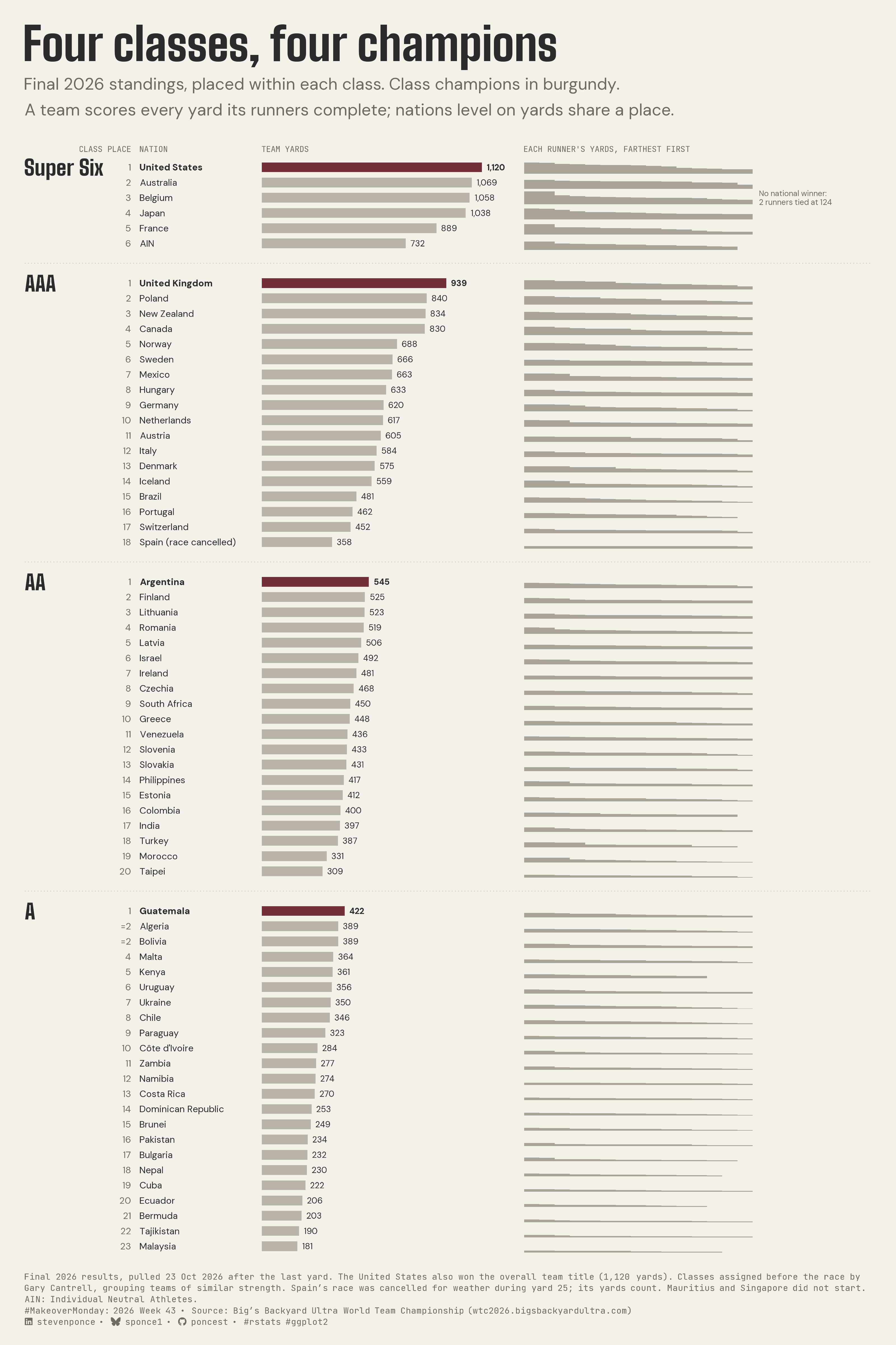
Final 2026 standings, placed within each class. Class champions in burgundy. A team scores every yard its runners complete; nations level on yards share a place.

MakeoverMonday

2026

A makeover of the 2026 Big’s Backyard Ultra World Team Championship standings, regrouping all 67 nations into the four pre-race classes and highlighting the class champions: United States, United Kingdom, Argentina and Guatemala. Places are recomputed within each class from team yards, with each nation’s runners shown as a sorted yards profile. Built in R with ggplot2, ggtext and showtext.

Author

Steven Ponce

Published

October 27, 2026

Original

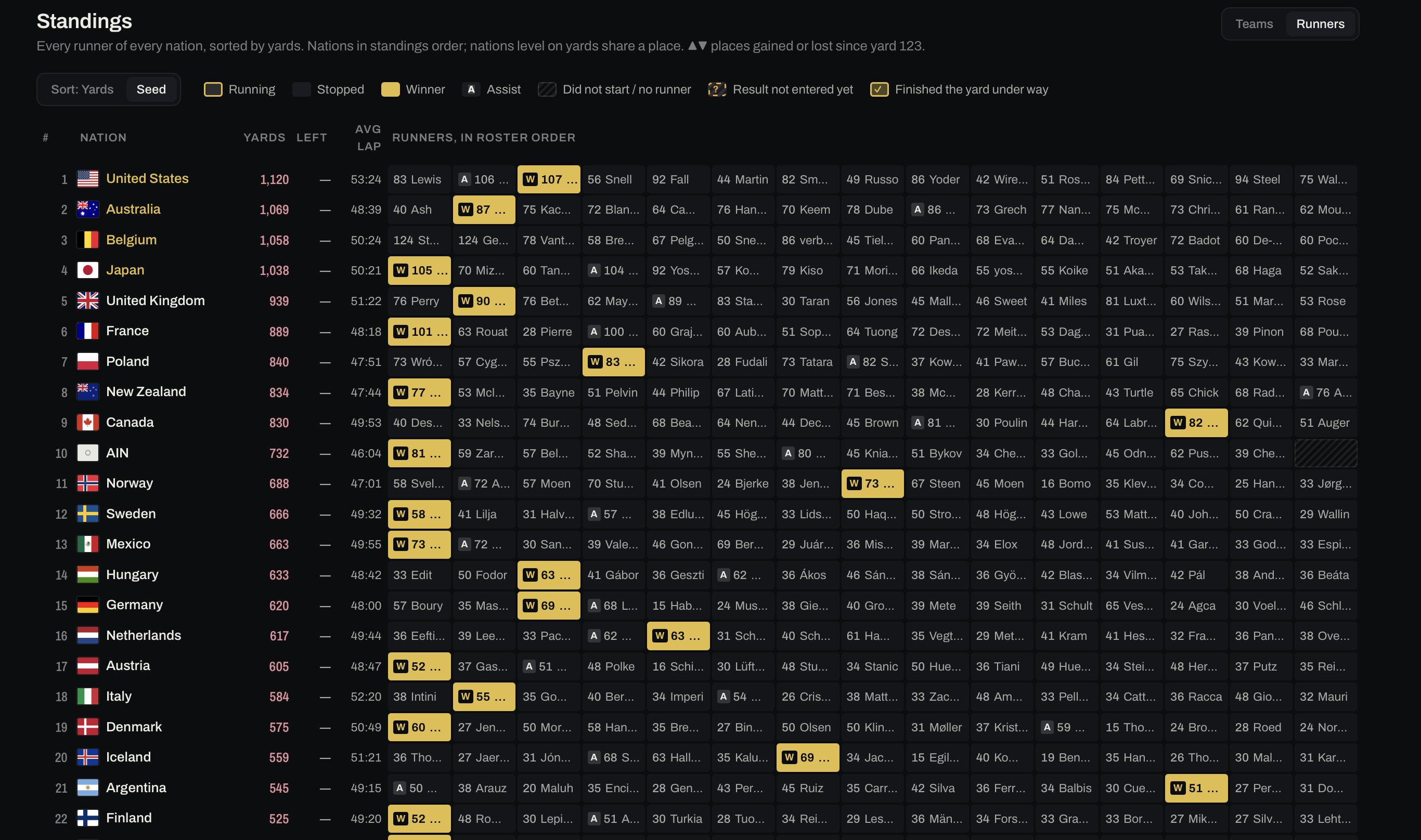
The original visualization comes from Big’s Backyard Ultramarathon World Team Championships

Makeover

Figure 1: A tall standings graphic titled “Four classes, four champions” shows the final 2026 Big’s Backyard Ultra World Team Championship results for 67 participating nations, organized into the four pre-race classes: Super Six, AAA, AA, and A. Each section lists nations by their place within the class. Horizontal bars show total team yards, with burgundy highlighting the four class champions: United States (1,120 yards, also the overall team champion), United Kingdom (939), Argentina (545) and Guatemala (422). To the right, small contiguous bars show each nation’s runners ordered from farthest to shortest. Belgium, third in the Super Six, has no national winner: its last two runners stopped together at 124 yards, the farthest anyone ran. Algeria and Bolivia share second place in class A with 389 yards each. Spain’s race was canceled due to weather during yard 25; its 358 yards still count. Source: Big’s Backyard Ultra World Team Championship.

Steps to Create this Graphic

1. Load Packages & Setup

Show code

```{r}
#| label: load
#| warning: false
#| message: false      
#| results: "hide"     

## 1. LOAD PACKAGES & SETUP ----
suppressPackageStartupMessages({
  if (!require("pacman")) install.packages("pacman")
  pacman::p_load(
    tidyverse, ggtext, showtext, scales, glue, 
  janitor, ggview, readxl, ggrepel, magick 
)
})

# Source utility functions
suppressMessages(
  source(here::here("R/utils/fonts.R")))
  source(here::here("R/utils/social_icons.R"))
  source(here::here("R/themes/base_theme.R"))

### |- figure size ----
fig_w <- 10
fig_h <- 15
fig_dpi <- 320

### |-  fonts ----
setup_fonts()
fonts <- get_font_families()
title_family <- fonts$title_1
text_family  <- fonts$text
cap_family   <- fonts$caption
```

2. Read in the Data

Show code

```{r}
#| label: read
#| include: true
#| eval: true
#| warning: false

xl_path <- here::here("data/MakeoverMonday/2026/bigs_backyard_wtc_2020_2026.xlsx")

read_sheet <- function(sheet_name) {
  read_excel(xl_path, sheet = sheet_name,
             col_types = "text", na = character()) |>
    clean_names()
}

df_runners <- read_sheet("runner_results")
df_nations <- read_sheet("nation_years")  
```

3. Examine the Data

Show code

```{r}
#| label: examine
#| include: true
#| eval: true
#| results: 'hide'
#| warning: false

glimpse(df_runners)
glimpse(df_nations)
df_nations |> filter(year == "2026") |> count(result_status)
```

4. Tidy Data

Show code

```{r}
#| label: tidy
#| warning: false

### |- standings: places rebuilt from team yards (site rule: level = shared place) ----
# The workbook's `rank` breaks 2026 ties by race distance; the site shares the
# place with no tie-break, and the site is the record. `rank` is never used.
class_levels <- c("SUPER" = "Super Six", "AAA" = "AAA", "AA" = "AA", "A" = "A")

standings <- df_nations |>
  filter(year == "2026", result_status %in% c("Final", "Cancelled")) |>
  mutate(
    team_yards    = as.numeric(team_yards),
    overall_place = min_rank(-team_yards),
    cancelled     = result_status == "Cancelled",
    division      = factor(class_levels[division_2026], levels = class_levels)
  ) |>
  mutate(
    place = min_rank(-team_yards),
    tied = duplicated(team_yards) | duplicated(team_yards, fromLast = TRUE),
    place_lab = if_else(tied, paste0("=", place), as.character(place)),
    champ = place == 1,
    .by = division
  ) |>
  mutate(
    nation_short = recode(nation, "United States of America" = "United States"),
    nation_lab   = if_else(cancelled, paste0(nation_short, " (race cancelled)"), nation_short)
  )

### |- runner profiles: starters only, sorted farthest to shortest ----
# DNS runners are left out, so a short team shows blank positions, not zeros
profiles <- df_runners |>
  filter(
    year == "2026", nation_code %in% standings$nation_code,
    result != "DNS"
  ) |>
  mutate(yards = as.numeric(yards)) |>
  arrange(nation_code, desc(yards)) |>
  mutate(pos = row_number(), .by = nation_code)

max_y <- max(profiles$yards)

# Each profile sums to its official team total (no 2026 nation is off by one)
prof_check <- profiles |>
  summarise(sum_y = sum(yards), .by = nation_code) |>
  left_join(standings |> select(nation_code, team_yards), by = "nation_code")

### |- layout: one numeric y, gaps between classes ----
gap <- 1.6

rows <- standings |>
  arrange(division, place, nation) |>
  mutate(
    seq   = row_number(),
    div_i = as.integer(division),
    y     = -(seq + (div_i - 1) * gap)
  )

class_lab <- rows |>
  summarise(y = max(y), .by = division) |>
  mutate(label = as.character(division))

dividers <- rows |>
  summarise(y_min = min(y), .by = div_i) |>
  filter(div_i < 4) |>
  mutate(y = y_min - (1 + gap) / 2)

# column positions (data units)
# class labels (Big Shoulders, ~10 units wide for "Super Six") get their own
# column; place starts after it so rank 1 is never covered
x_class <- 0
x_place <- 12.5
x_nation <- 13.6
x_bar0 <- 28
bar_len <- 26
x_prof0 <- 59
col_w <- 1.8
x_prof1 <- x_prof0 + 15 * col_w
x_note <- x_prof1 + 0.8
x_max <- 100
y_head <- 0.2

bars <- rows |>
  mutate(xmax = x_bar0 + bar_len * team_yards / max(team_yards))

prof_plot <- profiles |>
  inner_join(rows |> select(nation_code, y), by = "nation_code") |>
  mutate(
    xmin = x_prof0 + (pos - 1) * col_w,
    xmax = xmin + col_w,
    ymin = y - 0.42,
    ymax = y - 0.42 + 0.84 * yards / max_y
  )

bel_note <- rows |>
  filter(nation_code == "BEL") |>
  transmute(y, label = "No national winner:\n2 runners tied at 124")
```

5. Visualization Parameters

Show code

```{r}
#| label: params
#| include: true
#| warning: false

### |- plot aesthetics ----
colors <- get_theme_colors(
  palette = list(
    paper   = "#f4f1ea",
    ink     = "#2b2b2b",
    muted   = "#6f6a63",
    accent  = "#722F37",
    bar     = "#b9b3aa",
    profile = "#a9a297",
    rule    = "#cfc8be"
  )
)
clrs <- colors$palette
col_paper <- clrs$paper
col_ink <- clrs$ink
col_muted <- clrs$muted
col_accent <- clrs$accent
col_bar <- clrs$bar
col_profile <- clrs$profile
col_rule <- clrs$rule

### |- titles and caption ----
champs <- rows |>
  filter(champ) |>
  arrange(division)

title_text <- "Four classes, four champions"

subtitle_text <- paste0(
  "Final 2026 standings, placed within each class. Class champions in burgundy.\n",
  "A team scores every yard its runners complete; nations level on yards share a place."
)

note_text <- paste(
  "Final 2026 results, pulled 23 Oct 2026 after the last yard.",
  "The United States also won the overall team title (1,120 yards).",
  "Classes assigned before the race by Gary Cantrell, grouping teams of similar strength.",
  "Spain's race was cancelled for weather",
  "during yard 25; its yards count. Mauritius and Singapore did not start.",
  "AIN: Individual Neutral Athletes."
)

caption_text <- paste0(
  note_text, "<br>",
  create_mm_caption(
    mm_year = 2026,
    mm_week = 43,
    source_text = "Big's Backyard Ultra World Team Championship (wtc2026.bigsbackyardultra.com)"
  )
)

### |- plot theme ----
base_theme <- create_base_theme(colors)

weekly_theme <- extend_weekly_theme(
  base_theme,
  theme(
    plot.background = element_rect(fill = col_paper, colour = NA),
    panel.background = element_rect(fill = col_paper, colour = NA),
    panel.grid = element_blank(),
    axis.text = element_blank(),
    axis.title = element_blank(),
    axis.ticks = element_blank(),
    legend.position = "none",
    plot.title = element_text(
      family = title_family, size = rel(2.6), colour = col_ink,
      margin = margin(b = 6)
    ),
    plot.subtitle = element_text(
      family = text_family, size = rel(0.95), colour = col_muted,
      lineheight = 1.3, margin = margin(b = 14)
    ),
    plot.caption = element_textbox_simple(
      family = cap_family, size = rel(0.5), colour = col_muted,
      lineheight = 1.3, margin = margin(t = 12)
    ),
    plot.margin = margin(20, 20, 15, 20)
  )
)

theme_set(weekly_theme)
```

6. Plot

Show code

```{r}
#| label: plot
#| warning: false

### |-  main plot ----
p <- ggplot() +
  geom_segment(
    data = dividers,
    aes(x = x_class, xend = x_max, y = y, yend = y),
    colour = col_rule, linewidth = 0.3, linetype = "dotted"
  ) +
  annotate(
    "text",
    x = c(x_place, x_nation, x_bar0, x_prof0),
    y = y_head,
    label = c("CLASS PLACE", "NATION", "TEAM YARDS", "EACH RUNNER'S YARDS, FARTHEST FIRST"),
    hjust = c(1, 0, 0, 0),
    family = cap_family, size = 2.3, colour = col_muted
  ) +
  geom_text(
    data = class_lab,
    aes(x = x_class, y = y, label = label),
    hjust = 0, vjust = 0.5,
    family = title_family, size = 6, colour = col_ink
  ) +
  geom_text(
    data = rows,
    aes(x = x_place, y = y, label = place_lab),
    hjust = 1, family = text_family, size = 2.6, colour = col_muted
  ) +
  geom_text(
    data = rows,
    aes(
      x = x_nation, y = y, label = nation_lab,
      fontface = if_else(champ, "bold", "plain")
    ),
    hjust = 0, family = text_family, size = 2.6, colour = col_ink
  ) +
  geom_rect(
    data = bars,
    aes(
      xmin = x_bar0, xmax = xmax, ymin = y - 0.32, ymax = y + 0.32,
      fill = if_else(champ, col_accent, col_bar)
    )
  ) +
  geom_text(
    data = bars,
    aes(
      x = xmax + 0.6, y = y, label = comma(team_yards),
      fontface = if_else(champ, "bold", "plain")
    ),
    hjust = 0, family = text_family, size = 2.4, colour = col_ink
  ) +
  geom_rect(
    data = prof_plot,
    aes(xmin = xmin, xmax = xmax, ymin = ymin, ymax = ymax),
    fill = col_profile
  ) +
  geom_text(
    data = bel_note,
    aes(x = x_note, y = y, label = label),
    hjust = 0, vjust = 0.5, lineheight = 0.95,
    family = text_family, size = 2.2, colour = col_muted
  ) +
  scale_fill_identity() +
  coord_cartesian(
    xlim = c(x_class, x_max),
    ylim = c(min(rows$y) - 0.8, y_head + 0.8),
    expand = FALSE, clip = "off"
  ) +
  labs(title = title_text, subtitle = subtitle_text, caption = caption_text)
```

7. Save

Show code

```{r}
#| label: save
#| warning: false

### |- save ----
main_path  <- here::here("data_visualizations", "MakeoverMonday", "2026", "mm_2026_43.png")
thumb_path <- here::here("data_visualizations", "MakeoverMonday", "2026", "thumbnails", "mm_2026_43.png")

# Full-size version, for the QMD figure
save_ggplot(
  plot = p,
  file = main_path,
  width = fig_w, height = fig_h,
  units = "in", dpi = 320,
)

# Reduced-size thumbnail
fs::dir_create(dirname(thumb_path))
magick::image_read(main_path) |>
  magick::image_resize("400") |>
  magick::image_write(thumb_path)
```

8. Session Info

Expand for Session Info

R version 4.6.1 (2026-06-24)
Platform: aarch64-apple-darwin23
Running under: macOS Tahoe 26.6.2

Matrix products: default
BLAS:   /Library/Frameworks/R.framework/Versions/4.6/Resources/lib/libRblas.0.dylib 
LAPACK: /Library/Frameworks/R.framework/Versions/4.6/Resources/lib/libRlapack.dylib;  LAPACK version 3.12.1

locale:
[1] en_US.UTF-8/en_US.UTF-8/en_US.UTF-8/C/en_US.UTF-8/en_US.UTF-8

time zone: America/New_York
tzcode source: internal

attached base packages:
[1] stats     graphics  grDevices utils     datasets  methods   base     

other attached packages:
 [1] here_1.0.2      magick_2.9.1    ggrepel_0.9.8   readxl_1.5.0   
 [5] ggview_0.2.2    janitor_2.2.1   glue_1.8.1      scales_1.4.0   
 [9] showtext_0.9-8  showtextdb_3.0  sysfonts_0.8.9  ggtext_0.2.0   
[13] lubridate_1.9.5 forcats_1.0.1   stringr_1.6.0   dplyr_1.2.1    
[17] purrr_1.2.2     readr_2.2.0     tidyr_1.3.2     tibble_3.3.1   
[21] ggplot2_4.0.3   tidyverse_2.0.0 pacman_0.5.1   

loaded via a namespace (and not attached):
 [1] gtable_0.3.6       xfun_0.60          htmlwidgets_1.6.4  tzdb_0.5.0        
 [5] vctrs_0.7.3        tools_4.6.1        generics_0.1.4     curl_7.1.0        
 [9] pkgconfig_2.0.3    RColorBrewer_1.1-3 S7_0.2.2           lifecycle_1.0.5   
[13] compiler_4.6.1     farver_2.1.2       textshaping_1.0.5  codetools_0.2-20  
[17] snakecase_0.11.1   litedown_0.10      htmltools_0.5.9    yaml_2.3.12       
[21] pillar_1.11.1      commonmark_2.0.0   tidyselect_1.2.1   digest_0.6.39     
[25] stringi_1.8.7      labeling_0.4.3     rprojroot_2.1.1    fastmap_1.2.0     
[29] grid_4.6.1         cli_3.6.6          magrittr_2.0.5     utf8_1.2.6        
[33] withr_3.0.3        timechange_0.4.0   rmarkdown_2.31     otel_0.2.0        
[37] cellranger_1.1.0   ragg_1.5.2         hms_1.1.4          evaluate_1.0.5    
[41] knitr_1.51         markdown_2.0       rlang_1.3.0        gridtext_0.1.6    
[45] Rcpp_1.1.2         xml2_1.6.0         rstudioapi_0.19.0  jsonlite_2.0.0    
[49] R6_2.6.1           fs_2.1.0           systemfonts_1.3.2

9. GitHub Repository

Expand for GitHub Repo

The complete code for this analysis is available in mm_2026_43.qmd.

For the full repository, click here.

10. References

Expand for References

Primary Data (Makeover Monday): 1. Makeover Monday 2026 Week 43: Big’s Backyard Ultra World Team Championship - Workbook: a README plus three sheets: runner_yards (32,869 rows; one row per runner per completed yard, 2026 only), runner_results (2,830 rows; one row per runner, 2020–2026) and nation_years (190 rows; one row per nation per edition). This makeover uses the 2026 rows of runner_results and nation_years. - Coverage: final 2026 results, pulled 23 Oct 2026 after the last yard. 67 nations appear: 66 finished, and Spain’s race was cancelled for weather during yard 25 (its 358 yards stay in the standings). Mauritius and Singapore did not start and are not shown. - Places: recomputed from team yards within each class; nations level on yards share the place, with no tie-break (the site’s rule). The workbook’s rank column breaks 2026 ties by race distance and is not used. Overall ties: Brazil and Ireland (481, =27) and Algeria and Bolivia (389, =42); only Algeria and Bolivia share a class (=2 in class A). - Classes: assigned before the race by Gary Cantrell, grouping teams of similar strength: Super Six (6 nations), AAA (18), AA (20) and A (23). - Runner profiles: starters only (the 42 runners who did not start are left out, so short teams show blank positions), sorted farthest first, on one shared height scale (maximum 124 yards). Every nation’s profile sums exactly to its official team total. - Key figures: - Class champions: United States 1,120 (also the overall team title), United Kingdom 939, Argentina 545, Guatemala 422. - Belgium (3rd, Super Six) has no national winner: Merijn Geerts and Ivo Steyaert both completed 124 yards, the farthest anyone ran, and stopped together. - AIN: Individual Neutral Athletes (14 starters).

Source Data: 2. Big’s Backyard Ultra. World Team Championship 2026: results feed and official leaderboard. Race rules, classes and shared-place rule from the championship guide.

Original Visualization: 3. Big’s Backyard Ultra World Team Championship 2026, Standings: Runners view (live dashboard, app by Naresh Kumar): wtc2026.bigsbackyardultra.com.

Related Analysis: 4. Kumar, N. (2026). It takes fifteen and The middle wins. The source’s own analysis of team depth; this makeover redesigns the standings rather than repeating it.

11. Custom Functions Documentation

📦 Custom Helper Functions

This analysis uses custom functions from my personal module library for efficiency and consistency across projects.

Functions Used:

fonts.R: setup_fonts(), get_font_families() - Font management with showtext
social_icons.R: create_social_caption() - Generates formatted social media captions
image_utils.R: save_plot() - Consistent plot saving with naming conventions
base_theme.R: create_base_theme(), extend_weekly_theme(), get_theme_colors() - Custom ggplot2 themes

Why custom functions?
These utilities standardize theming, fonts, and output across all my data visualizations. The core analysis (data tidying and visualization logic) uses only standard tidyverse packages.

Source Code:
View all custom functions → GitHub: R/utils

Citation

BibTeX citation:

@online{ponce2026,
  author = {Ponce, Steven},
  title = {Four Classes, Four Champions},
  date = {2026-10-27},
  url = {https://stevenponce.netlify.app/data_visualizations/MakeoverMonday/2026/mm_2026_43.html},
  langid = {en}
}

For attribution, please cite this work as:

Ponce, Steven. 2026. “Four Classes, Four Champions.” October 27. https://stevenponce.netlify.app/data_visualizations/MakeoverMonday/2026/mm_2026_43.html.

--- title: "Four classes, four champions" subtitle: "Final 2026 standings, placed within each class. Class champions in burgundy. A team scores every yard its runners complete; nations level on yards share a place." description: "A makeover of the 2026 Big's Backyard Ultra World Team Championship standings, regrouping all 67 nations into the four pre-race classes and highlighting the class champions: United States, United Kingdom, Argentina and Guatemala. Places are recomputed within each class from team yards, with each nation's runners shown as a sorted yards profile. Built in R with ggplot2, ggtext and showtext." date: "2026-10-27" author: - name: "Steven Ponce" url: "https://stevenponce.netlify.app" citation: url: "https://stevenponce.netlify.app/data_visualizations/MakeoverMonday/2026/mm_2026_43.html" categories: ["MakeoverMonday", "2026"] tags: [ "makeover-monday", "data-visualization", "ggplot2", "ultramarathon", "backyard-ultra", "sports", "standings-table", "bar-chart", "small-bars", "ranking", "ties", "ggtext", "showtext", "2026" ] image: "thumbnails/mm_2026_43.png" format: html: toc: true toc-depth: 5 code-link: true code-fold: true code-tools: true code-summary: "Show code" editor_options: chunk_output_type: inline execute: freeze: true cache: true error: false message: false warning: false eval: true --- ```{r} #| label: setup-links #| include: false # CENTRALIZED LINK MANAGEMENT ## Project-specific info current_year <- 2026 current_week <- 43 project_file <- "mm_2026_43.qmd" project_image <- "mm_2026_43.png" ## Data Sources data_main <- "https://wtc2026.bigsbackyardultra.com" data_secondary <- "https://wtc2026.bigsbackyardultra.com" ## Repository Links repo_main <- "https://github.com/poncest/personal-website/" repo_file <- paste0("https://github.com/poncest/personal-website/blob/master/data_visualizations/MakeoverMonday/", current_year, "/", project_file) ## External Resources/Images chart_original <- "https://raw.githubusercontent.com/poncest/MakeoverMonday/refs/heads/master/2026/Week_43/original_chart.png" ## Organization/Platform Links org_primary <- "https://wtc2026.bigsbackyardultra.com" org_secondary <- "https://wtc2026.bigsbackyardultra.com" # Helper function to create markdown links create_link <- function(text, url) { paste0("[", text, "](", url, ")") } # Helper function for citation-style links create_citation_link <- function(text, url, title = NULL) { if (is.null(title)) { paste0("[", text, "](", url, ")") } else { paste0("[", text, "](", url, ' "', title, '")') } } ``` ### Original The original visualization comes from `r create_link("Big's Backyard Ultramarathon World Team Championships", org_primary)` ![Original visualization](https://raw.githubusercontent.com/poncest/MakeoverMonday/refs/heads/master/2026/Week_43/original_chart.png) ### Makeover ![A tall standings graphic titled "Four classes, four champions" shows the final 2026 Big's Backyard Ultra World Team Championship results for 67 participating nations, organized into the four pre-race classes: Super Six, AAA, AA, and A. Each section lists nations by their place within the class. Horizontal bars show total team yards, with burgundy highlighting the four class champions: United States (1,120 yards, also the overall team champion), United Kingdom (939), Argentina (545) and Guatemala (422). To the right, small contiguous bars show each nation's runners ordered from farthest to shortest. Belgium, third in the Super Six, has no national winner: its last two runners stopped together at 124 yards, the farthest anyone ran. Algeria and Bolivia share second place in class A with 389 yards each. Spain's race was canceled due to weather during yard 25; its 358 yards still count. Source: Big's Backyard Ultra World Team Championship.](mm_2026_43.png){#fig-1} ### [**Steps to Create this Graphic**]{.mark} #### [1. Load Packages & Setup]{.smallcaps} ```{r} #| label: load #| warning: false #| message: false #| results: "hide" ## 1. LOAD PACKAGES & SETUP ---- suppressPackageStartupMessages({ if (!require("pacman")) install.packages("pacman") pacman::p_load( tidyverse, ggtext, showtext, scales, glue, janitor, ggview, readxl, ggrepel, magick ) }) # Source utility functions suppressMessages( source(here::here("R/utils/fonts.R"))) source(here::here("R/utils/social_icons.R")) source(here::here("R/themes/base_theme.R")) ### |- figure size ---- fig_w <- 10 fig_h <- 15 fig_dpi <- 320 ### |- fonts ---- setup_fonts() fonts <- get_font_families() title_family <- fonts$title_1 text_family <- fonts$text cap_family <- fonts$caption ``` #### [2. Read in the Data]{.smallcaps} ```{r} #| label: read #| include: true #| eval: true #| warning: false xl_path <- here::here("data/MakeoverMonday/2026/bigs_backyard_wtc_2020_2026.xlsx") read_sheet <- function(sheet_name) { read_excel(xl_path, sheet = sheet_name, col_types = "text", na = character()) |> clean_names() } df_runners <- read_sheet("runner_results") df_nations <- read_sheet("nation_years") ``` #### [3. Examine the Data]{.smallcaps} ```{r} #| label: examine #| include: true #| eval: true #| results: 'hide' #| warning: false glimpse(df_runners) glimpse(df_nations) df_nations |> filter(year == "2026") |> count(result_status) ``` #### [4. Tidy Data]{.smallcaps} ```{r} #| label: tidy #| warning: false ### |- standings: places rebuilt from team yards (site rule: level = shared place) ---- # The workbook's `rank` breaks 2026 ties by race distance; the site shares the # place with no tie-break, and the site is the record. `rank` is never used. class_levels <- c("SUPER" = "Super Six", "AAA" = "AAA", "AA" = "AA", "A" = "A") standings <- df_nations |> filter(year == "2026", result_status %in% c("Final", "Cancelled")) |> mutate( team_yards = as.numeric(team_yards), overall_place = min_rank(-team_yards), cancelled = result_status == "Cancelled", division = factor(class_levels[division_2026], levels = class_levels) ) |> mutate( place = min_rank(-team_yards), tied = duplicated(team_yards) | duplicated(team_yards, fromLast = TRUE), place_lab = if_else(tied, paste0("=", place), as.character(place)), champ = place == 1, .by = division ) |> mutate( nation_short = recode(nation, "United States of America" = "United States"), nation_lab = if_else(cancelled, paste0(nation_short, " (race cancelled)"), nation_short) ) ### |- runner profiles: starters only, sorted farthest to shortest ---- # DNS runners are left out, so a short team shows blank positions, not zeros profiles <- df_runners |> filter( year == "2026", nation_code %in% standings$nation_code, result != "DNS" ) |> mutate(yards = as.numeric(yards)) |> arrange(nation_code, desc(yards)) |> mutate(pos = row_number(), .by = nation_code) max_y <- max(profiles$yards) # Each profile sums to its official team total (no 2026 nation is off by one) prof_check <- profiles |> summarise(sum_y = sum(yards), .by = nation_code) |> left_join(standings |> select(nation_code, team_yards), by = "nation_code") ### |- layout: one numeric y, gaps between classes ---- gap <- 1.6 rows <- standings |> arrange(division, place, nation) |> mutate( seq = row_number(), div_i = as.integer(division), y = -(seq + (div_i - 1) * gap) ) class_lab <- rows |> summarise(y = max(y), .by = division) |> mutate(label = as.character(division)) dividers <- rows |> summarise(y_min = min(y), .by = div_i) |> filter(div_i < 4) |> mutate(y = y_min - (1 + gap) / 2) # column positions (data units) # class labels (Big Shoulders, ~10 units wide for "Super Six") get their own # column; place starts after it so rank 1 is never covered x_class <- 0 x_place <- 12.5 x_nation <- 13.6 x_bar0 <- 28 bar_len <- 26 x_prof0 <- 59 col_w <- 1.8 x_prof1 <- x_prof0 + 15 * col_w x_note <- x_prof1 + 0.8 x_max <- 100 y_head <- 0.2 bars <- rows |> mutate(xmax = x_bar0 + bar_len * team_yards / max(team_yards)) prof_plot <- profiles |> inner_join(rows |> select(nation_code, y), by = "nation_code") |> mutate( xmin = x_prof0 + (pos - 1) * col_w, xmax = xmin + col_w, ymin = y - 0.42, ymax = y - 0.42 + 0.84 * yards / max_y ) bel_note <- rows |> filter(nation_code == "BEL") |> transmute(y, label = "No national winner:\n2 runners tied at 124") ``` #### [5. Visualization Parameters]{.smallcaps} ```{r} #| label: params #| include: true #| warning: false ### |- plot aesthetics ---- colors <- get_theme_colors( palette = list( paper = "#f4f1ea", ink = "#2b2b2b", muted = "#6f6a63", accent = "#722F37", bar = "#b9b3aa", profile = "#a9a297", rule = "#cfc8be" ) ) clrs <- colors$palette col_paper <- clrs$paper col_ink <- clrs$ink col_muted <- clrs$muted col_accent <- clrs$accent col_bar <- clrs$bar col_profile <- clrs$profile col_rule <- clrs$rule ### |- titles and caption ---- champs <- rows |> filter(champ) |> arrange(division) title_text <- "Four classes, four champions" subtitle_text <- paste0( "Final 2026 standings, placed within each class. Class champions in burgundy.\n", "A team scores every yard its runners complete; nations level on yards share a place." ) note_text <- paste( "Final 2026 results, pulled 23 Oct 2026 after the last yard.", "The United States also won the overall team title (1,120 yards).", "Classes assigned before the race by Gary Cantrell, grouping teams of similar strength.", "Spain's race was cancelled for weather", "during yard 25; its yards count. Mauritius and Singapore did not start.", "AIN: Individual Neutral Athletes." ) caption_text <- paste0( note_text, "<br>", create_mm_caption( mm_year = 2026, mm_week = 43, source_text = "Big's Backyard Ultra World Team Championship (wtc2026.bigsbackyardultra.com)" ) ) ### |- plot theme ---- base_theme <- create_base_theme(colors) weekly_theme <- extend_weekly_theme( base_theme, theme( plot.background = element_rect(fill = col_paper, colour = NA), panel.background = element_rect(fill = col_paper, colour = NA), panel.grid = element_blank(), axis.text = element_blank(), axis.title = element_blank(), axis.ticks = element_blank(), legend.position = "none", plot.title = element_text( family = title_family, size = rel(2.6), colour = col_ink, margin = margin(b = 6) ), plot.subtitle = element_text( family = text_family, size = rel(0.95), colour = col_muted, lineheight = 1.3, margin = margin(b = 14) ), plot.caption = element_textbox_simple( family = cap_family, size = rel(0.5), colour = col_muted, lineheight = 1.3, margin = margin(t = 12) ), plot.margin = margin(20, 20, 15, 20) ) ) theme_set(weekly_theme) ``` #### [6. Plot]{.smallcaps} ```{r} #| label: plot #| warning: false ### |- main plot ---- p <- ggplot() + geom_segment( data = dividers, aes(x = x_class, xend = x_max, y = y, yend = y), colour = col_rule, linewidth = 0.3, linetype = "dotted" ) + annotate( "text", x = c(x_place, x_nation, x_bar0, x_prof0), y = y_head, label = c("CLASS PLACE", "NATION", "TEAM YARDS", "EACH RUNNER'S YARDS, FARTHEST FIRST"), hjust = c(1, 0, 0, 0), family = cap_family, size = 2.3, colour = col_muted ) + geom_text( data = class_lab, aes(x = x_class, y = y, label = label), hjust = 0, vjust = 0.5, family = title_family, size = 6, colour = col_ink ) + geom_text( data = rows, aes(x = x_place, y = y, label = place_lab), hjust = 1, family = text_family, size = 2.6, colour = col_muted ) + geom_text( data = rows, aes( x = x_nation, y = y, label = nation_lab, fontface = if_else(champ, "bold", "plain") ), hjust = 0, family = text_family, size = 2.6, colour = col_ink ) + geom_rect( data = bars, aes( xmin = x_bar0, xmax = xmax, ymin = y - 0.32, ymax = y + 0.32, fill = if_else(champ, col_accent, col_bar) ) ) + geom_text( data = bars, aes( x = xmax + 0.6, y = y, label = comma(team_yards), fontface = if_else(champ, "bold", "plain") ), hjust = 0, family = text_family, size = 2.4, colour = col_ink ) + geom_rect( data = prof_plot, aes(xmin = xmin, xmax = xmax, ymin = ymin, ymax = ymax), fill = col_profile ) + geom_text( data = bel_note, aes(x = x_note, y = y, label = label), hjust = 0, vjust = 0.5, lineheight = 0.95, family = text_family, size = 2.2, colour = col_muted ) + scale_fill_identity() + coord_cartesian( xlim = c(x_class, x_max), ylim = c(min(rows$y) - 0.8, y_head + 0.8), expand = FALSE, clip = "off" ) + labs(title = title_text, subtitle = subtitle_text, caption = caption_text) ``` #### [7. Save]{.smallcaps} ```{r} #| label: save #| warning: false ### |- save ---- main_path <- here::here("data_visualizations", "MakeoverMonday", "2026", "mm_2026_43.png") thumb_path <- here::here("data_visualizations", "MakeoverMonday", "2026", "thumbnails", "mm_2026_43.png") # Full-size version, for the QMD figure save_ggplot( plot = p, file = main_path, width = fig_w, height = fig_h, units = "in", dpi = 320, ) # Reduced-size thumbnail fs::dir_create(dirname(thumb_path)) magick::image_read(main_path) |> magick::image_resize("400") |> magick::image_write(thumb_path) ``` #### [8. Session Info]{.smallcaps} ::: {.callout-tip collapse="true"} ##### Expand for Session Info ```{r, echo = FALSE} #| eval: true #| warning: false sessionInfo() ``` ::: #### [9. GitHub Repository]{.smallcaps} ::: {.callout-tip collapse="true"} ##### Expand for GitHub Repo The complete code for this analysis is available in `r create_link(project_file, repo_file)`. For the full repository, `r create_link("click here", repo_main)`. ::: #### [10. References]{.smallcaps} ::: {.callout-tip collapse="true"} ##### Expand for References **Primary Data (Makeover Monday):** 1. Makeover Monday 2026 Week 43: `r create_link("Big's Backyard Ultra World Team Championship", "https://wtc2026.bigsbackyardultra.com")` - Workbook: a README plus three sheets: `runner_yards` (32,869 rows; one row per runner per completed yard, 2026 only), `runner_results` (2,830 rows; one row per runner, 2020–2026) and `nation_years` (190 rows; one row per nation per edition). This makeover uses the 2026 rows of `runner_results` and `nation_years`. - **Coverage:** final 2026 results, pulled 23 Oct 2026 after the last yard. 67 nations appear: 66 finished, and Spain's race was cancelled for weather during yard 25 (its 358 yards stay in the standings). Mauritius and Singapore did not start and are not shown. - **Places:** recomputed from team yards *within each class*; nations level on yards share the place, with no tie-break (the site's rule). The workbook's `rank` column breaks 2026 ties by race distance and is not used. Overall ties: Brazil and Ireland (481, =27) and Algeria and Bolivia (389, =42); only Algeria and Bolivia share a class (=2 in class A). - **Classes:** assigned before the race by Gary Cantrell, grouping teams of similar strength: Super Six (6 nations), AAA (18), AA (20) and A (23). - **Runner profiles:** starters only (the 42 runners who did not start are left out, so short teams show blank positions), sorted farthest first, on one shared height scale (maximum 124 yards). Every nation's profile sums exactly to its official team total. - **Key figures:** - Class champions: United States 1,120 (also the overall team title), United Kingdom 939, Argentina 545, Guatemala 422. - Belgium (3rd, Super Six) has no national winner: Merijn Geerts and Ivo Steyaert both completed 124 yards, the farthest anyone ran, and stopped together. - AIN: Individual Neutral Athletes (14 starters). **Source Data:** 2. Big's Backyard Ultra. `r create_link("World Team Championship 2026: results feed and official leaderboard", "https://wtc2026.bigsbackyardultra.com")`. Race rules, classes and shared-place rule from the `r create_link("championship guide", "https://wtc2026.bigsbackyardultra.com/guide")`. **Original Visualization:** 3. Big's Backyard Ultra World Team Championship 2026, *Standings: Runners* view (live dashboard, app by Naresh Kumar): `r create_link("wtc2026.bigsbackyardultra.com", "https://wtc2026.bigsbackyardultra.com")`. **Related Analysis:** 4. Kumar, N. (2026). `r create_link("It takes fifteen", "https://wtc2026.bigsbackyardultra.com/story")` and `r create_link("The middle wins", "https://wtc2026.bigsbackyardultra.com/story-2026")`. The source's own analysis of team depth; this makeover redesigns the standings rather than repeating it. ::: #### [11. Custom Functions Documentation]{.smallcaps} ::: {.callout-note collapse="true"} ##### 📦 Custom Helper Functions This analysis uses custom functions from my personal module library for efficiency and consistency across projects. **Functions Used:** - **`fonts.R`**: `setup_fonts()`, `get_font_families()` - Font management with showtext - **`social_icons.R`**: `create_social_caption()` - Generates formatted social media captions - **`image_utils.R`**: `save_plot()` - Consistent plot saving with naming conventions - **`base_theme.R`**: `create_base_theme()`, `extend_weekly_theme()`, `get_theme_colors()` - Custom ggplot2 themes **Why custom functions?**\ These utilities standardize theming, fonts, and output across all my data visualizations. The core analysis (data tidying and visualization logic) uses only standard tidyverse packages. **Source Code:**\ View all custom functions → [GitHub: R/utils](https://github.com/poncest/personal-website/tree/master/R) :::