---
title: "The top science systems differ unusually widely in student AI use"
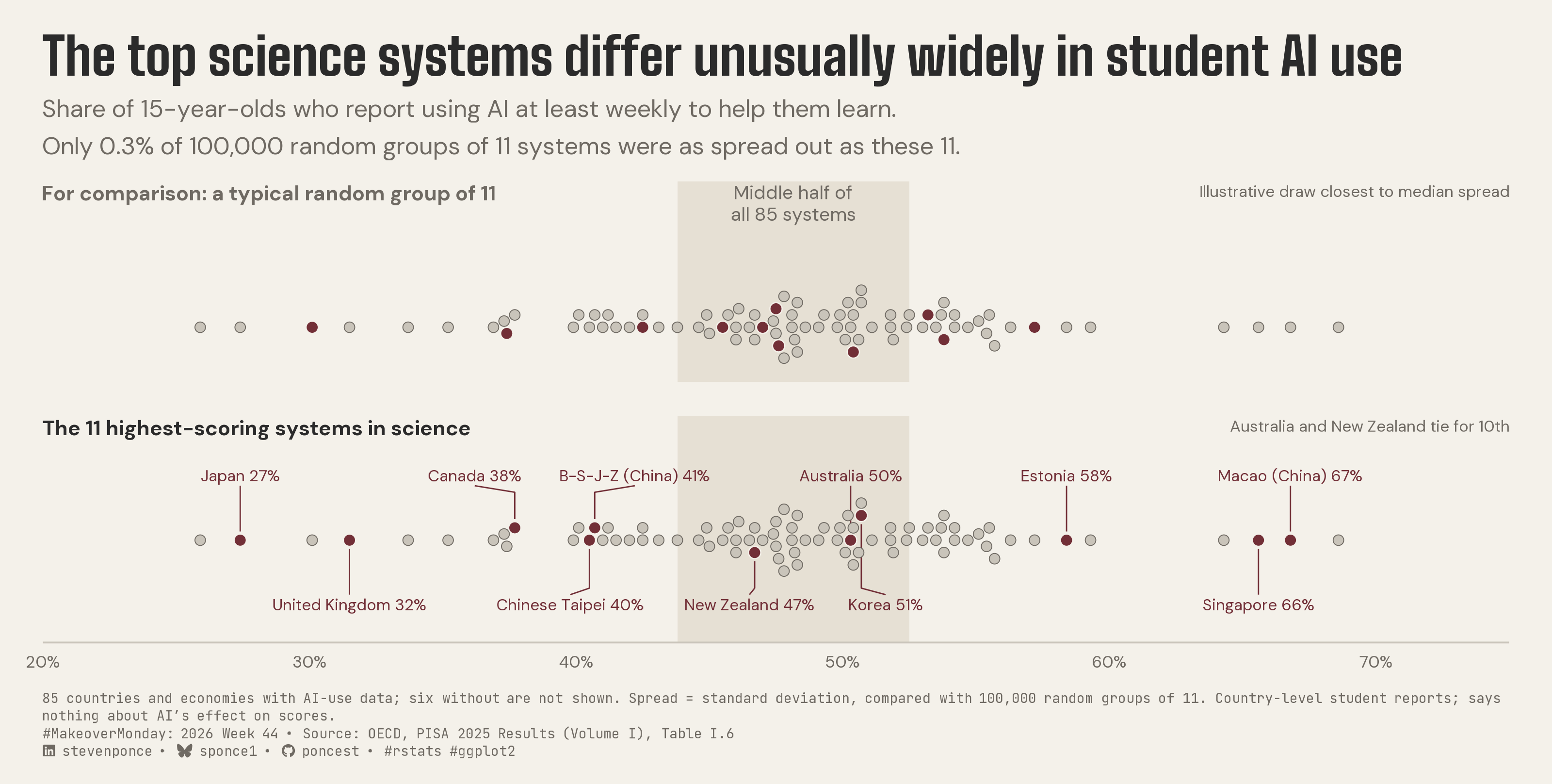
subtitle: "Share of 15-year-olds who report using AI at least weekly to help them learn. Only 0.3% of 100,000 random groups of 11 systems were as spread out as these 11."
description: "Among the 11 highest-scoring PISA 2025 science systems, the share of students using AI weekly ranges from 27% to 67%, more spread out than 99.7% of random groups of 11. A two-panel dot strip compares them with an illustrative random group drawn from the same 85 countries and economies. Built in R with ggplot2, ggtext and showtext."
date: "2026-11-01"
author:
- name: "Steven Ponce"
url: "https://stevenponce.netlify.app"
citation:
url: "https://stevenponce.netlify.app/data_visualizations/MakeoverMonday/2026/mm_2026_44.html"
categories: ["MakeoverMonday", "2026"]
tags: [
"makeover-monday",
"pisa",
"oecd",
"education",
"artificial-intelligence",
"ai-in-education",
"beeswarm",
"dot-strip",
"random-baseline",
"variation",
"ggplot2",
"ggtext",
"showtext",
"2026"
]
image: "thumbnails/mm_2026_44.png"
format:
html:
toc: true
toc-depth: 5
code-link: true
code-fold: true
code-tools: true
code-summary: "Show code"
editor_options:
chunk_output_type: inline
execute:
freeze: true
cache: true
error: false
message: false
warning: false
eval: true
---
```{r}
#| label: setup-links
#| include: false
# CENTRALIZED LINK MANAGEMENT
## Weekly inputs (the only lines to edit) ----
current_year <- 2026
current_week <- 44
mm_slug <- "pisa-2025"
source_article <- "https://www.oecd.org/en/publications/pisa-2025-results-volume-i_73451bc5-en.html" # SOURCE ARTICLE on the MM page
data_source <- "https://www.oecd.org/en/publications/pisa-2025-results-volume-i_73451bc5-en.html" # DATA SOURCE on the MM page
## Derived (don't edit) ----
project_id <- sprintf("mm_%d_%02d", current_year, current_week)
project_file <- paste0(project_id, ".qmd")
mm_page <- paste0("https://makeovermonday.vercel.app/dataset/", mm_slug)
chart_original <- sprintf(
"https://raw.githubusercontent.com/poncest/MakeoverMonday/refs/heads/master/%d/Week_%02d/original_chart.png",
current_year, current_week
)
repo_main <- "https://github.com/poncest/personal-website/"
repo_file <- paste0(
repo_main, "blob/master/data_visualizations/MakeoverMonday/",
current_year, "/", project_file
)
## Helper ----
create_link <- function(text, url) paste0("[", text, "](", url, ")")
```
### Original
The original visualization comes from `r create_link("PISA 2025 Results (Volume I)", source_article)`.

### Makeover
{#fig-1}
### [**Steps to Create this Graphic**]{.mark}
#### [1. Load Packages & Setup]{.smallcaps}
```{r}
#| label: load
#| warning: false
#| message: false
#| results: "hide"

## 1. LOAD PACKAGES & SETUP ----
suppressPackageStartupMessages({
  if (!require("pacman")) install.packages("pacman")
  pacman::p_load(
    tidyverse, ggtext, showtext, scales, glue,
  janitor, ggview, readxl, ggrepel, magick
)
})

# Source utility functions
suppressMessages(
  source(here::here("R/utils/fonts.R")))
  source(here::here("R/utils/social_icons.R"))
  source(here::here("R/themes/base_theme.R"))

### |- figure size ----
fig_w <- 10
fig_h <- 5.05
fig_dpi <- 320

### |-  fonts ----
setup_fonts()
fonts <- get_font_families()
title_family <- fonts$title_1
text_family <- fonts$text
cap_family <- fonts$caption
```
#### [2. Read in the Data]{.smallcaps}
```{r}
#| label: read
#| include: true
#| eval: true
#| warning: false

xl_path <- here::here("data/MakeoverMonday/2026/PISA2025.xlsx")

read_sheet <- function(sheet_name) {
  read_excel(xl_path,
    sheet = sheet_name,
    col_types = "text", na = character()
  ) |>
    clean_names()
}

df_raw <- read_sheet("PISA2025-Data")
```
#### [3. Examine the Data]{.smallcaps}
```{r}
#| label: examine
#| include: true
#| eval: true
#| results: 'hide'
#| warning: false

glimpse(df_raw)
```
#### [4. Tidy Data]{.smallcaps}
```{r}
#| label: tidy
#| warning: false

### |- one row per system with weekly-AI data ----
df <- df_raw |>
  transmute(
    country,
    sci    = as.numeric(science_mean_score),
    ai_pct = 100 * as.numeric(students_using_ai_at_least_weekly_to_help_them_learn)
  ) |>
  filter(!is.na(ai_pct)) |>
  mutate(id = row_number())

n_sys <- nrow(df)

### |- top group: tie-preserving cut at the 10th science score ----
# Australia and New Zealand tie at 509 for 10th place; a top-10 cut would drop
# one of them on an arbitrary tie-break, so the group keeps every system >= 509
k_target <- 10
cut_sci <- sort(df$sci, decreasing = TRUE)[k_target]
top_set <- df |> filter(sci >= cut_sci)
n_top <- nrow(top_set)

### |- random-group comparison (the test behind the subtitle) ----
# Spread = standard deviation of a group's shares. 100,000 random groups of
# n_top systems are drawn from the 85; the share at least as spread out as the
# top group is the reported rate.
n_draws <- 100000
set.seed(2044)
draws <- replicate(n_draws, sample.int(n_sys, n_top)) # n_top x n_draws
draw_sd <- apply(matrix(df$ai_pct[draws], nrow = n_top), 2, sd)

top_sd <- sd(top_set$ai_pct)
median_sd <- median(draw_sd)
share_ge <- mean(draw_sd >= top_sd)

# illustrative group: the draw whose spread is closest to the median (first on
# ties) -- fixed by rule, never chosen by how it looks
pick <- which.min(abs(draw_sd - median_sd))
rand_ids <- draws[, pick]

share_lab <- paste0(format(round(100 * share_ge, 1), nsmall = 1), "%")

### |- middle half of all 85 systems (the reference band) ----
q_lo <- unname(quantile(df$ai_pct, 0.25))
q_hi <- unname(quantile(df$ai_pct, 0.75))
n_top_in_band <- sum(top_set$ai_pct >= q_lo & top_set$ai_pct <= q_hi)

### |- beeswarm, computed once in physical points ----
x_lim <- c(20, 75)
panel_w_in <- fig_w - 2 * 20 / 72
pt_per_pct <- panel_w_in * 72 / diff(x_lim)
dot_size <- 2.1
d_pt <- dot_size * .pt * 0.75 + 1.2

swarm_y <- function(x_pt, d) {
  ord <- order(x_pt)
  y <- numeric(length(x_pt))
  placed <- integer(0)
  offsets <- c(0, as.vector(rbind(seq_len(80), -seq_len(80))) * d * 0.5)
  for (i in ord) {
    for (cand in offsets) {
      if (length(placed) == 0 ||
        all((x_pt[i] - x_pt[placed])^2 + (cand - y[placed])^2 >= d^2)) {
        y[i] <- cand
        break
      }
    }
    placed <- c(placed, i)
  }
  y
}

df <- df |> mutate(y = swarm_y(ai_pct * pt_per_pct, d_pt))
y_max <- max(abs(df$y))
row_gap <- 10

# Each panel gets only the height it needs (same pt-per-unit scale in both):
# upper = heading + band label + swarm; lower = heading + two label rows + swarm
head_clear <- 16 # heading block height + gap above the next element (pt)
band_clear <- 28 # two-line band label + gap above the swarm (pt)
label_h <- 10 # one label line (pt)
axis_clear <- 10 # gap between the bottom label row and the axis (pt)

panel_lims <- tibble(
  panel = c("random", "top"),
  y_lo = c(-(y_max + 8), -(y_max + row_gap + label_h + axis_clear)),
  y_hi = c(
    y_max + 6 + band_clear + head_clear,
    y_max + row_gap + label_h + head_clear + 4
  )
)

y_range_total <- sum(panel_lims$y_hi - panel_lims$y_lo)

panel_levels <- c("random", "top")

plot_df <- bind_rows(
  df |> mutate(panel = "random", hi = id %in% rand_ids),
  df |> mutate(panel = "top", hi = id %in% top_set$id)
) |>
  mutate(panel = factor(panel, levels = panel_levels))

### |- labels for the top group----
label_size <- 2.6
char_pct <- label_size * .pt * 0.60 / pt_per_pct

nudge_row <- function(x, w, gap = 0.8) {
  for (iter in 1:200) {
    moved <- FALSE
    for (i in seq_along(x)[-1]) {
      need <- (w[i - 1] + w[i]) / 2 + gap
      if (x[i] - x[i - 1] < need) {
        push <- (need - (x[i] - x[i - 1])) / 2
        x[i - 1] <- x[i - 1] - push
        x[i] <- x[i] + push
        moved <- TRUE
      }
    }
    if (!moved) break
  }
  x
}

labels_df <- df |>
  filter(id %in% top_set$id) |>
  arrange(ai_pct) |>
  mutate(
    label = glue("{country} {round(ai_pct)}%"),
    side  = if_else(row_number() %% 2 == 1, 1, -1),
    panel = factor("top", levels = panel_levels)
  ) |>
  group_by(side) |>
  mutate(label_x = nudge_row(ai_pct, nchar(label) * char_pct)) |>
  ungroup() |>
  mutate(
    label_y = side * (y_max + row_gap),
    vjust   = if_else(side > 0, 0, 1)
  )

leaders <- labels_df |>
  mutate(label_id = row_number()) |>
  reframe(
    x = c(ai_pct, ai_pct, label_x),
    y = c(y + side * 4, label_y - side * 5, label_y - side * 2),
    .by = c(label_id, panel)
  )
```
#### [5. Visualization Parameters]{.smallcaps}
```{r}
#| label: params
#| include: true
#| warning: false

### |- plot aesthetics ----
colors <- get_theme_colors(
  palette = list(
    paper  = "#f4f1ea",
    ink    = "#2b2b2b",
    muted  = "#6f6a63",
    accent = "#722F37",
    dot    = "#c9c4ba",
    band   = "#e6e0d4"
  )
)
clrs <- colors$palette
col_paper <- clrs$paper
col_ink <- clrs$ink
col_muted <- clrs$muted
col_accent <- clrs$accent
col_dot <- clrs$dot
col_band <- clrs$band

### |- titles and caption ----
title_text <- "The top science systems differ unusually widely in student AI use"

subtitle_text <- paste0(
  "Share of 15-year-olds who report using AI at least weekly to help them learn.\n",
  glue("Only {share_lab} of {comma(n_draws)} random groups of {n_top} systems were as spread out as these {n_top}.")
)

headings <- tibble(
  panel = factor(panel_levels, levels = panel_levels),
  label = c(
    glue("For comparison: a typical random group of {n_top}"),
    glue("The {n_top} highest-scoring systems in science")
  ),
  colour = c(col_muted, col_ink),
  x = x_lim[1],
  y = panel_lims$y_hi - 2
)

# right-aligned notes, one per panel: how each highlighted group was chosen
panel_notes <- tibble(
  panel = factor(panel_levels, levels = panel_levels),
  x = x_lim[2],
  y = panel_lims$y_hi - 2,
  label = c(
    "Illustrative draw closest to median spread",
    "Australia and New Zealand tie for 10th"
  )
)

band_lab <- tibble(
  panel = factor("random", levels = panel_levels),
  x = (q_lo + q_hi) / 2,
  y = panel_lims$y_hi[1] - 2,
  label = glue("Middle half of\nall {n_sys} systems")
)

note_text <- paste(
  glue("{n_sys} countries and economies with AI-use data; six without are not shown."),
  glue("Spread = standard deviation, compared with {comma(n_draws)} random groups of {n_top}."),
  "Country-level student reports; says nothing about AI's effect on scores."
)

caption_text <- paste0(
  note_text, "<br>",
  create_mm_caption(
    mm_year = 2026,
    mm_week = 44,
    source_text = "OECD, PISA 2025 Results (Volume I), Table I.6"
  )
)

### |- plot theme ----
base_theme <- create_base_theme(colors)

weekly_theme <- extend_weekly_theme(
  base_theme,
  theme(
    plot.background = element_rect(fill = col_paper, colour = NA),
    panel.background = element_rect(fill = col_paper, colour = NA),
    panel.grid = element_blank(),
    axis.text.y = element_blank(),
    axis.text.x = element_text(family = text_family, size = rel(0.7), colour = col_muted),
    axis.title = element_blank(),
    axis.ticks = element_blank(),
    axis.line.x = element_line(colour = col_dot, linewidth = 0.4),
    strip.text = element_blank(),
    panel.spacing = unit(16, "pt"),
    legend.position = "none",
    plot.title = element_text(
      family = title_family, size = rel(1.72), colour = col_ink,
      margin = margin(b = 6)
    ),
    plot.subtitle = element_text(
      family = text_family, size = rel(0.80), colour = col_muted,
      lineheight = 1.3, margin = margin(b = 10)
    ),
    plot.caption = element_textbox_simple(
      family = cap_family, size = rel(0.45), colour = col_muted,
      lineheight = 1.3, margin = margin(t = 10)
    ),
    plot.margin = margin(16, 20, 12, 20)
  )
)

theme_set(weekly_theme)
```
#### [6. Plot]{.smallcaps}
```{r}
#| label: plot
#| warning: false

### |-  main plot ----
p <- ggplot(plot_df, aes(x = ai_pct, y = y)) +
  annotate(
    "rect", xmin = q_lo, xmax = q_hi, ymin = -Inf, ymax = Inf,
    fill = col_band
  ) +
  geom_path(
    data = leaders, aes(x = x, y = y, group = label_id),
    colour = col_accent, linewidth = 0.3
  ) +
  geom_point(
    data = filter(plot_df, !hi),
    shape = 21, size = dot_size, fill = col_dot, colour = col_muted, stroke = 0.3
  ) +
  geom_point(
    data = filter(plot_df, hi),
    shape = 21, size = dot_size + 0.3, fill = col_accent, colour = col_paper, stroke = 0.4
  ) +
  geom_text(
    data = labels_df,
    aes(x = label_x, y = label_y, label = label, vjust = vjust),
    family = text_family, size = label_size, colour = col_accent
  ) +
  geom_text(
    data = headings,
    aes(x = x, y = y, label = label, colour = colour),
    hjust = 0, vjust = 1, fontface = "bold",
    family = text_family, size = 3.4
  ) +
  geom_text(
    data = panel_notes,
    aes(x = x, y = y, label = label),
    hjust = 1, vjust = 1,
    family = text_family, size = 2.6, colour = col_muted
  ) +
  geom_text(
    data = band_lab,
    aes(x = x, y = y, label = label),
    vjust = 1, lineheight = 0.95,
    family = text_family, size = 3.1, colour = col_muted
  ) +
  scale_colour_identity() +
  scale_x_continuous(breaks = seq(20, 70, 10), labels = label_percent(scale = 1)) +
  geom_blank(
    data = panel_lims |>
      mutate(panel = factor(panel, levels = panel_levels)) |>
      pivot_longer(c(y_lo, y_hi), values_to = "y") |>
      mutate(ai_pct = mean(x_lim)),
    aes(x = ai_pct, y = y)
  ) +
  scale_y_continuous(expand = expansion(0)) +
  facet_grid(panel ~ ., scales = "free_y", space = "free_y") +
  coord_cartesian(xlim = x_lim, expand = FALSE, clip = "off") +
  labs(title = title_text, subtitle = subtitle_text, caption = caption_text)
```
#### [7. Save]{.smallcaps}
```{r}
#| label: save
#| warning: false

### |- save ----
main_path  <- here::here("data_visualizations", "MakeoverMonday", "2026", "mm_2026_44.png")
thumb_path <- here::here("data_visualizations", "MakeoverMonday", "2026", "thumbnails", "mm_2026_44.png")

# Full-size version, for the QMD figure
save_ggplot(
  plot = p,
  file = main_path,
  width = fig_w, height = fig_h,
  units = "in", dpi = 320,
)

# Reduced-size thumbnail
fs::dir_create(dirname(thumb_path))
magick::image_read(main_path) |>
  magick::image_resize("400") |>
  magick::image_write(thumb_path)
```
#### [8. Session Info]{.smallcaps}
::: {.callout-tip collapse="true"}
##### Expand for Session Info
```{r, echo = FALSE}
#| eval: true
#| warning: false
sessionInfo()
```
:::
#### [9. GitHub Repository]{.smallcaps}
::: {.callout-tip collapse="true"}
##### Expand for GitHub Repo
The complete code for this analysis is available in `r create_link(project_file, repo_file)`.
For the full repository, `r create_link("click here", repo_main)`.
:::
#### [10. References]{.smallcaps}
::: {.callout-tip collapse="true"}
##### Expand for References
**Primary Data (Makeover Monday):**
1. Makeover Monday `r current_year` Week `r current_week`: `r create_link("PISA 2025: Digital learning, AI and student performance", mm_page)`
- Workbook: 91 countries and economies, 19 fields, extracted from Tables I.1 and I.6 of the report; 85 have weekly-AI-use data (Cambodia, Dushanbe, Kurdistan Region, Mauritius, Rwanda and Zambia do not).
- Region and OECD-member columns were added by the dataset author; the About sheet cites an OECD-average sheet that is not in the file.
- Change since 2022 carries no significance flags; Uzbekistan's +83 in science is flagged by the source as needing care.
**Source Data:**
2. OECD (2026). *PISA 2025 Results (Volume I): Future-Ready Students*. OECD Publishing, Paris. `r create_link("https://doi.org/10.1787/73451bc5-en", data_source)`. Table I.6 (snapshot of digitalisation and AI); Table I.1 (performance). CC BY 4.0.
**Original Visualization:**
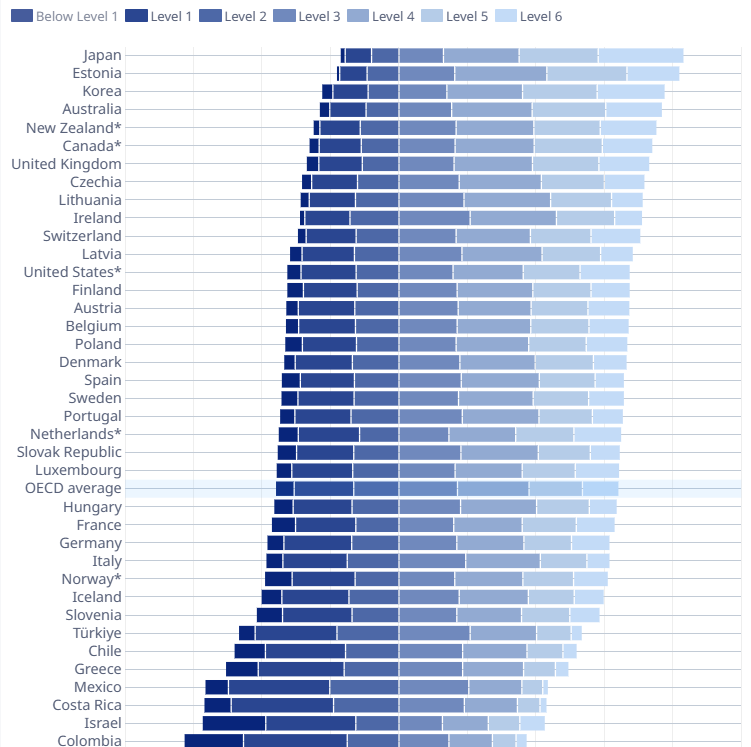
3. OECD (2026), *PISA 2025 Results (Volume I)*: science proficiency levels for OECD countries, a seven-band diverging bar chart centred on Level 2. `r create_link("OECD publication page", source_article)`.
**Related Analysis:**
4. OECD (2026). `r create_link("Executive Summary, PISA 2025 Results (Volume I)", "https://read.oecd-ilibrary.org/en/publications/pisa-2025-results-volume-i_73451bc5-en/full-report/executive-summary_3701b0ef.html")`. The source reports AI findings at the student level: students who use AI for specific schoolwork score lower, and weekly general users score about the same as non-users. This makeover works at the country level and makes no claim about effects.
**Analysis Frame:**
- **Measure:** share of 15-year-olds who report using AI at least weekly to help them learn (student questionnaire, country-level).
- **Top group:** the 11 systems scoring 509 or higher in science. Australia and New Zealand tie at 509 for 10th, so both are included rather than broken by an arbitrary tie-break.
- **Comparison:** standard deviation of the top group's shares (13.0 points) against 100,000 random groups of 11 drawn from the 85 (median 7.7). 0.28% were as spread out (seed 2044).
- **Upper panel:** the random draw whose spread is closest to that median. It illustrates a typical group; it is not the test.
- **Reference band:** middle half of all 85 systems, 43.8% to 52.5%; 3 of the 11 fall inside it.
:::
#### [11. Custom Functions Documentation]{.smallcaps}
::: {.callout-note collapse="true"}
##### 📦 Custom Helper Functions
This analysis uses custom functions from my personal module library for efficiency and consistency across projects.
**Functions Used:**
- **`fonts.R`**: `setup_fonts()`, `get_font_families()` - Font management with showtext
- **`social_icons.R`**: `create_social_caption()` - Generates formatted social media captions
- **`image_utils.R`**: `save_plot()` - Consistent plot saving with naming conventions
- **`base_theme.R`**: `create_base_theme()`, `extend_weekly_theme()`, `get_theme_colors()` - Custom ggplot2 themes
**Why custom functions?**\
These utilities standardize theming, fonts, and output across all my data visualizations. The core analysis (data tidying and visualization logic) uses only standard tidyverse packages.
**Source Code:**\
View all custom functions → [GitHub: R/utils](https://github.com/poncest/personal-website/tree/master/R)
:::