The typical balloon stayed the same size. Giants became more common.

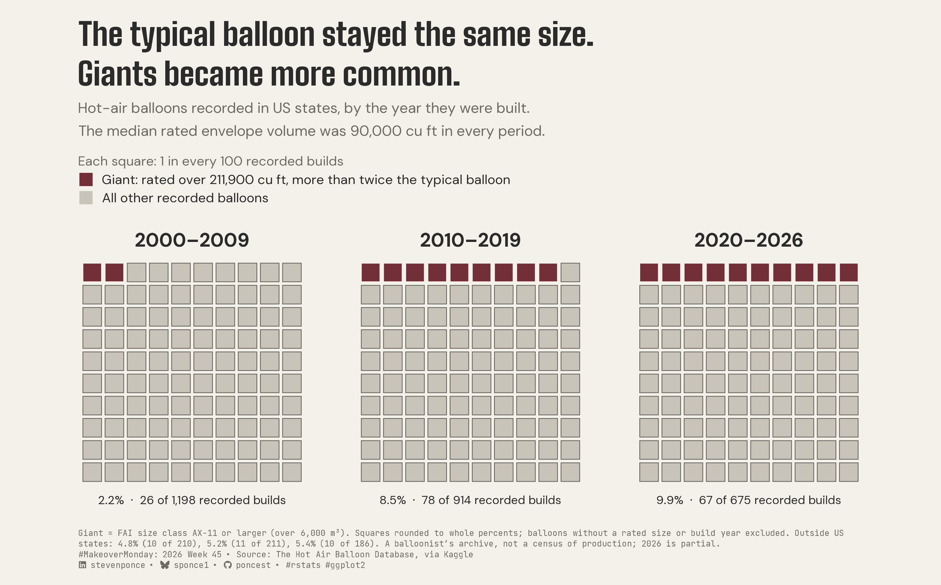
Hot-air balloons recorded in US states, by the year they were built. The median rated envelope volume was 90,000 cu ft in every period.

MakeoverMonday

2026

Among hot-air balloons recorded in US states, giants rated over 211,900 cu ft rose from 2.2% of builds in 2000–2009 to 8.5% in 2010–2019 and 9.9% in 2020–2026, while the median stayed at 90,000 cu ft. Each period is shown as a per-100 unit grid, with giants defined by the FAI AX-11 size class. Built in R with ggplot2, ggtext and showtext.

Author

Steven Ponce

Published

November 9, 2026

Original

The original visualization comes from Hot Air Balloons.

Makeover

Figure 1: Three-panel unit chart titled “The typical balloon stayed the same size. Giants became more common.” Each panel is a 10-by-10 grid in which every square stands for 1 in every 100 hot-air balloons recorded in US states, grouped by build period; burgundy squares mark giants, rated over 211,900 cubic feet, more than twice the typical balloon. Giants rose from 2 squares in 2000–2009 (2.2%, 26 of 1,198 recorded builds) to 9 in 2010–2019 (8.5%, 78 of 914) and a full top row of 10 in 2020–2026 (9.9%, 67 of 675), with most of the rise coming in the 2010s. The median rated envelope volume stayed at 90,000 cubic feet in every period. Outside the US, the giant share stayed near 5%. Data: The Hot Air Balloon Database, via Kaggle; 2026 is a partial year.

Steps to Create this Graphic

1. Load Packages & Setup

Show code

```{r}
#| label: load
#| warning: false
#| message: false      
#| results: "hide"     

## 1. LOAD PACKAGES & SETUP ----
suppressPackageStartupMessages({
  if (!require("pacman")) install.packages("pacman")
  pacman::p_load(
    tidyverse, ggtext, showtext, scales, glue, 
  janitor, ggview, readxl, magick, janitor
)
})

# Source utility functions
suppressMessages(
  source(here::here("R/utils/fonts.R")))
  source(here::here("R/utils/social_icons.R"))
  source(here::here("R/themes/base_theme.R"))

### |- figure size ----
fig_w <- 10
fig_dpi <- 320
fig_h <- 6.22

### |-  fonts ----
setup_fonts()
fonts <- get_font_families()
title_family <- fonts$title_1
text_family <- fonts$text
cap_family <- fonts$caption
```

2. Read in the Data

Show code

```{r}
#| label: read
#| include: true
#| eval: true
#| warning: false

xl_path <- here::here("data/MakeoverMonday/2026/hot_air_balloon.xlsx")

df_raw <- read_excel(
  xl_path,
  skip = 1,
  col_types = "text",
  na = character(),
  .name_repair = "unique"
) |>
  clean_names()
```

3. Examine the Data

Show code

```{r}
#| label: examine
#| include: true
#| eval: true
#| results: 'hide'
#| warning: false

# split records
df_raw <- df_raw |>
  mutate(
    is_record = str_detect(balloon_id, "^HAB-\\d{6}$"),
    record_no = cumsum(is_record)
  )

glimpse(df_raw)
```

4. Tidy Data

Show code

```{r}
#| label: tidy
#| warning: false

### |- reattach the split records ----
fragments <- df_raw |>
  filter(!is_record) |>
  summarise(
    owners_cont = paste(balloon_id, collapse = " "),
    across(c(name, registration, manufacturer, model, serial_number, year_built, size), last),
    .by = record_no
  ) |>
  mutate(
    record_no, owners_cont,
    image_f = name, seen_f = registration, crewed_f = manufacturer,
    flown_f = model, burner_time_f = serial_number,
    additional_images_f = year_built, notes_f = size,
    .keep = "none"
  )

balloons <- df_raw |>
  filter(is_record) |>
  left_join(fragments, by = "record_no") |>
  mutate(
    previous_owners = if_else(is.na(owners_cont), previous_owners,
      str_squish(paste(previous_owners, owners_cont))
    ),
    image = coalesce(image_f, image),
    seen = coalesce(seen_f, seen),
    crewed = coalesce(crewed_f, crewed),
    flown = coalesce(flown_f, flown),
    burner_time = coalesce(burner_time_f, burner_time),
    additional_images = coalesce(additional_images_f, additional_images),
    notes = coalesce(notes_f, notes)
  ) |>
  select(balloon_id:notes)

### |- parse fields ----
balloons <- balloons |>
  mutate(
    # first four-digit year = original build; 4 impossible values (2969, 2997 x2,
    # 6077) and 3 malformed ones ("200", "2-14", "2-22") become NA
    build_year = suppressWarnings(as.integer(str_extract(year_built, "^\\d{4}"))),
    build_year = if_else(build_year > 2026, NA_integer_, build_year),
    volume_cuft = suppressWarnings(as.numeric(
      str_remove_all(str_extract(size, "^[\\d,]+(?=\\s*cu)"), ",")
    )),
    in_us_state = location %in% c(state.name, "District of Columbia")
  )

### |- giant threshold: FAI size class AX-11 and above ----
# FAI Sporting Code Section 1 (Aug 2026), 2.1.2: category 11 = 6,000-9,000 m3
cuft_per_m3 <- 35.3147
giant_m3 <- 6000
giant_cuft <- giant_m3 * cuft_per_m3

### |- the three build periods compared ----
periods <- tibble(
  period = c("2000–2009", "2010–2019", "2020–2026"),
  from   = c(2000L, 2010L, 2020L),
  to     = c(2009L, 2019L, 2026L)
)

sized <- balloons |>
  filter(!is.na(volume_cuft), !is.na(build_year)) |>
  inner_join(periods, by = join_by(between(build_year, from, to))) |>
  mutate(giant = volume_cuft > giant_cuft)

us_summary <- sized |>
  filter(in_us_state) |>
  summarise(
    n = n(), k = sum(giant), median_cuft = median(volume_cuft),
    .by = period
  ) |>
  arrange(period) |>
  mutate(
    pct   = 100 * k / n,
    units = round(pct)
  )

outside_summary <- sized |>
  filter(!in_us_state) |>
  summarise(n = n(), k = sum(giant), .by = period) |>
  arrange(period) |>
  mutate(pct = 100 * k / n)

typical_cuft <- unique(us_summary$median_cuft)

### |- unit grids: 10 x 10 per period ----
grid_df <- us_summary |>
  select(period, units) |>
  reframe(i = 1:100, .by = c(period, units)) |>
  mutate(
    col  = (i - 1) %% 10,
    row  = 9 - (i - 1) %/% 10,
    kind = factor(if_else(i <= units, "giant", "other"), levels = c("giant", "other"))
  )

grid_labels <- us_summary |>
  mutate(
    label = glue("{sprintf('%.1f', pct)}%  ·  {k} of {comma(n)} recorded builds"),
    x = 4.5, y = -1.25
  )
```

5. Visualization Parameters

Show code

```{r}
#| label: params
#| include: true
#| warning: false

### |- plot aesthetics ----
colors <- get_theme_colors(
  palette = list(
    paper  = "#f4f1ea",
    ink    = "#2b2b2b",
    muted  = "#6f6a63",
    accent = "#722F37",
    square = "#c9c4ba"
  )
)
clrs <- colors$palette
col_paper <- clrs$paper
col_ink <- clrs$ink
col_muted <- clrs$muted
col_accent <- clrs$accent
col_square <- clrs$square

### |- titles and caption ----
title_text <- "The typical balloon stayed the same size.\nGiants became more common."

subtitle_text <- paste0(
  "Hot-air balloons recorded in US states, by the year they were built.\n",
  glue("The median rated envelope volume was {comma(typical_cuft)} cu ft in every period.")
)

key_labels <- c(
  giant = glue("Giant: rated over {comma(round(giant_cuft, -2))} cu ft, more than twice the typical balloon"),
  other = "All other recorded balloons"
)

note_text <- paste(
  glue("Giant = FAI size class AX-11 or larger (over {comma(giant_m3)} m³)."),
  "Squares rounded to whole percents; balloons without a rated size or build year excluded.",
  glue(
    "Outside US states: ",
    paste(glue("{sprintf('%.1f', outside_summary$pct)}% ({outside_summary$k} of {outside_summary$n})"), collapse = ", "),
    "."
  ),
  "A balloonist's archive, not a census of production; 2026 is partial."
)

caption_text <- paste0(
  note_text, "<br>",
  create_mm_caption(
    mm_year = 2026,
    mm_week = 45,
    source_text = "The Hot Air Balloon Database, via Kaggle"
  )
)

### |- plot theme ----
base_theme <- create_base_theme(colors)

weekly_theme <- extend_weekly_theme(
  base_theme,
  theme(
    plot.background = element_rect(fill = col_paper, colour = NA),
    panel.background = element_rect(fill = col_paper, colour = NA),
    panel.grid = element_blank(),
    axis.text = element_blank(),
    axis.title = element_blank(),
    axis.ticks = element_blank(),
    strip.text = element_text(
      family = text_family, face = "bold", size = rel(1.05),
      colour = col_ink, margin = margin(b = 8)
    ),
    panel.spacing = unit(40, "pt"),
    legend.position = "top",
    legend.justification = "left",
    legend.direction = "vertical",
    legend.title = element_text(
      family = text_family, size = rel(0.72), colour = col_muted,
      margin = margin(b = 4)
    ),
    legend.text = element_text(family = text_family, size = rel(0.72), colour = col_ink),
    legend.key.size = unit(11, "pt"),
    legend.key.spacing.y = unit(3, "pt"),
    legend.margin = margin(t = 2, b = 6),
    plot.title = element_text(
      family = title_family, size = rel(1.72), colour = col_ink,
      lineheight = 1.05, margin = margin(b = 8)
    ),
    plot.subtitle = element_text(
      family = text_family, size = rel(0.80), colour = col_muted,
      lineheight = 1.3, margin = margin(b = 10)
    ),
    plot.caption = element_textbox_simple(
      family = cap_family, size = rel(0.45), colour = col_muted,
      lineheight = 1.3, margin = margin(t = 12)
    ),
    plot.margin = margin(16, 60, 12, 60)
  )
)

theme_set(weekly_theme)
```

6. Plot

Show code

```{r}
#| label: plot
#| warning: false

### |-  main plot ----
p <- ggplot(grid_df, aes(x = col, y = row)) +
  geom_tile(
    aes(fill = kind, colour = kind),
    width = 0.84, height = 0.84, linewidth = 0.3
  ) +
  geom_text(
    data = grid_labels,
    aes(x = x, y = y, label = label),
    family = text_family, size = 3.2, colour = col_ink
  ) +
  scale_fill_manual(
    values = c(giant = col_accent, other = col_square),
    labels = key_labels,
    name = "Each square: 1 in every 100 recorded builds"
  ) +
  scale_colour_manual(
    values = c(giant = col_paper, other = col_muted),
    guide = "none"
  ) +
  scale_x_continuous(limits = c(-0.6, 9.6), expand = expansion(0)) +
  scale_y_continuous(limits = c(-1.9, 9.6), expand = expansion(0)) +
  facet_wrap(~period) +
  coord_fixed(clip = "off") +
  labs(title = title_text, subtitle = subtitle_text, caption = caption_text)
```

7. Save

Show code

```{r}
#| label: save
#| warning: false

### |- save ----
main_path  <- here::here("data_visualizations", "MakeoverMonday", "2026", "mm_2026_45.png")
thumb_path <- here::here("data_visualizations", "MakeoverMonday", "2026", "thumbnails", "mm_2026_45.png")

# Full-size version, for the QMD figure
save_ggplot(
  plot = p,
  file = main_path,
  width = fig_w, height = fig_h,
  units = "in", dpi = 320,
)

# Reduced-size thumbnail
fs::dir_create(dirname(thumb_path))
magick::image_read(main_path) |>
  magick::image_resize("400") |>
  magick::image_write(thumb_path)
```

8. Session Info

Expand for Session Info

R version 4.6.1 (2026-06-24)
Platform: aarch64-apple-darwin23
Running under: macOS Tahoe 26.7.2

Matrix products: default
BLAS:   /Library/Frameworks/R.framework/Versions/4.6/Resources/lib/libRblas.0.dylib 
LAPACK: /Library/Frameworks/R.framework/Versions/4.6/Resources/lib/libRlapack.dylib;  LAPACK version 3.12.1

locale:
[1] en_US.UTF-8/en_US.UTF-8/en_US.UTF-8/C/en_US.UTF-8/en_US.UTF-8

time zone: America/New_York
tzcode source: internal

attached base packages:
[1] stats     graphics  grDevices utils     datasets  methods   base     

other attached packages:
 [1] here_1.0.2      magick_2.9.1    readxl_1.5.0    ggview_0.2.2   
 [5] janitor_2.2.1   glue_1.8.1      scales_1.4.0    showtext_0.9-8 
 [9] showtextdb_3.0  sysfonts_0.8.9  ggtext_0.2.0    lubridate_1.9.5
[13] forcats_1.0.1   stringr_1.6.0   dplyr_1.2.1     purrr_1.2.2    
[17] readr_2.2.0     tidyr_1.3.2     tibble_3.3.1    ggplot2_4.0.3  
[21] tidyverse_2.0.0 pacman_0.5.1   

loaded via a namespace (and not attached):
 [1] gtable_0.3.6       xfun_0.60          htmlwidgets_1.6.4  tzdb_0.5.0        
 [5] vctrs_0.7.3        tools_4.6.1        generics_0.1.4     curl_7.1.0        
 [9] pkgconfig_2.0.3    RColorBrewer_1.1-3 S7_0.2.2           lifecycle_1.0.5   
[13] compiler_4.6.1     farver_2.1.2       textshaping_1.0.5  codetools_0.2-20  
[17] snakecase_0.11.1   litedown_0.10      htmltools_0.5.9    yaml_2.3.12       
[21] pillar_1.11.1      commonmark_2.0.0   tidyselect_1.2.1   digest_0.6.39     
[25] stringi_1.8.7      labeling_0.4.3     rprojroot_2.1.1    fastmap_1.2.0     
[29] grid_4.6.1         cli_3.6.6          magrittr_2.0.5     withr_3.0.3       
[33] timechange_0.4.0   rmarkdown_2.31     otel_0.2.0         cellranger_1.1.0  
[37] ragg_1.5.2         hms_1.1.4          evaluate_1.0.5     knitr_1.51        
[41] markdown_2.0       rlang_1.3.0        gridtext_0.1.6     Rcpp_1.1.2        
[45] xml2_1.6.0         rstudioapi_0.19.0  jsonlite_2.0.0     R6_2.6.1          
[49] fs_2.1.0           systemfonts_1.3.2

9. GitHub Repository

Expand for GitHub Repo

The complete code for this analysis is available in mm_2026_45.qmd.

For the full repository, click here.

10. References

Expand for References

Primary Data (Makeover Monday): 1. Makeover Monday 2026 Week 45: Hot Air Balloons - Workbook: one sheet, 7,934 rows × 22 fields below a title row. A line break inside the previous-owners field split 412 records across 699 extra rows; rebuilt, the file holds 7,235 balloons (IDs HAB-000001 to HAB-007235, none missing), matching the archive’s own counter, and 55 manufacturers, also matching. - Build year parses for 6,920 balloons (the first year listed; rebuild dates ignored; seven impossible or malformed values treated as missing). - Size is the model’s rated envelope volume in cubic feet, taken from the catalog, not measured per balloon.

Source Data: 2. The Hot Air Balloon Database. thehabdatabase.com, via Kaggle (matthuff4): Hot Air Balloon dataset. A community archive of recorded balloons, not a census of production; snapshot date not stated.

Original Visualization: 3. The Hot Air Balloon Database homepage: three counters (“7,235 balloons documented”, “55 manufacturers represented”, “6,205 pilots & owners connected”). The first two are reproduced exactly from the file; the third could not be reproduced, because its definition isn’t stated, so it is not used.

Classification: 4. FAI (2026). Sporting Code Section 1 – Aerostats, version 3.0, effective 1 August 2026, para 2.1.2: size category 11 = 6,000 to 9,000 m³. 5. Cameron Balloons. A-Type envelope specifications: the A-210 (210,000 cu ft) is AX-10 and the A-225 (225,000 cu ft) is AX-11, consistent with the 6,000 m³ boundary.

Analysis Frame: - Population: balloons recorded in US states (50 states plus DC) with a rated size and a build year. - Periods: 2000–2009, 2010–2019 and 2020–2026 (2026 is partial). Earlier decades are thinly recorded in the archive and are not shown. - Giant: rated over 6,000 m³ (211,888 cu ft), FAI class AX-11 or larger; more than twice the median. Near the line, only three rated volumes occur: 210,000 (AX-10), 211,000 (Raven/Aerostar S-77A, still AX-10) and 225,000 (AX-11). - Shares: 26 of 1,198 (2.2%), 78 of 914 (8.5%) and 67 of 675 (9.9%). The grids round these to whole percents: 2, 9 and 10 squares. - Typical balloon: median rated volume of 90,000 cu ft in all three periods. - Outside US states: 10 of 210 (4.8%), 11 of 211 (5.2%) and 10 of 186 (5.4%). - Scope: counts describe the archive’s records, not the market. The chart makes no claim about why giants became more common.

11. Custom Functions Documentation

📦 Custom Helper Functions

This analysis uses custom functions from my personal module library for efficiency and consistency across projects.

Functions Used:

fonts.R: setup_fonts(), get_font_families() - Font management with showtext
social_icons.R: create_social_caption() - Generates formatted social media captions
base_theme.R: create_base_theme(), extend_weekly_theme(), get_theme_colors() - Custom ggplot2 themes

Why custom functions?
These utilities standardize theming, fonts, and output across all my data visualizations. The core analysis (data tidying and visualization logic) uses only standard tidyverse packages.

Source Code:
View all custom functions → GitHub: R/utils

Citation

BibTeX citation:

@online{ponce2026,
  author = {Ponce, Steven},
  title = {The Typical Balloon Stayed the Same Size. {Giants} Became
    More Common.},
  date = {2026-11-09},
  url = {https://stevenponce.netlify.app/data_visualizations/MakeoverMonday/2026/mm_2026_45.html},
  langid = {en}
}

For attribution, please cite this work as:

Ponce, Steven. 2026. “The Typical Balloon Stayed the Same Size. Giants Became More Common.” November 9. https://stevenponce.netlify.app/data_visualizations/MakeoverMonday/2026/mm_2026_45.html.

--- title: "The typical balloon stayed the same size. Giants became more common." subtitle: "Hot-air balloons recorded in US states, by the year they were built. The median rated envelope volume was 90,000 cu ft in every period." description: "Among hot-air balloons recorded in US states, giants rated over 211,900 cu ft rose from 2.2% of builds in 2000–2009 to 8.5% in 2010–2019 and 9.9% in 2020–2026, while the median stayed at 90,000 cu ft. Each period is shown as a per-100 unit grid, with giants defined by the FAI AX-11 size class. Built in R with ggplot2, ggtext and showtext." date: "2026-11-09" author: - name: "Steven Ponce" url: "https://stevenponce.netlify.app" citation: url: "https://stevenponce.netlify.app/data_visualizations/MakeoverMonday/2026/mm_2026_45.html" categories: ["MakeoverMonday", "2026"] tags: [ "makeover-monday", "ggplot2", "ggtext", "showtext", "waffle-chart", "unit-chart", "proportions", "hot-air-balloons", "ballooning", "aviation", "archival-data", "kpi-makeover", "2026" ] image: "thumbnails/mm_2026_45.png" format: html: toc: true toc-depth: 5 code-link: true code-fold: true code-tools: true code-summary: "Show code" editor_options: chunk_output_type: inline execute: freeze: true cache: true error: false message: false warning: false eval: true editor: markdown: wrap: sentence --- ```{r} #| label: setup-links #| include: false # CENTRALIZED LINK MANAGEMENT ## Weekly inputs (the only lines to edit) ---- current_year <- 2026 current_week <- 45 mm_slug <- "hot-air-balloons" source_article <- "https://thehabdatabase.com" # SOURCE ARTICLE on the MM page data_source <- "https://www.kaggle.com/datasets/matthuff4/hot-air-balloon" # DATA SOURCE on the MM page ## Derived (don't edit) ---- project_id <- sprintf("mm_%d_%02d", current_year, current_week) project_file <- paste0(project_id, ".qmd") mm_page <- paste0("https://makeovermonday.vercel.app/dataset/", mm_slug) chart_original <- sprintf( "https://raw.githubusercontent.com/poncest/MakeoverMonday/refs/heads/master/%d/Week_%02d/original_chart.png", current_year, current_week) repo_main <- "https://github.com/poncest/personal-website/" repo_file <- paste0( repo_main, "blob/master/data_visualizations/MakeoverMonday/", current_year, "/", project_file ) ## Helper ---- create_link <- function(text, url) paste0("[", text, "](", url, ")") ``` ### Original The original visualization comes from `r create_link("Hot Air Balloons", source_article)`. ![Original visualization](https://raw.githubusercontent.com/poncest/MakeoverMonday/refs/heads/master/2026/Week_45/original_chart.png) ### Makeover ![Three-panel unit chart titled "The typical balloon stayed the same size. Giants became more common." Each panel is a 10-by-10 grid in which every square stands for 1 in every 100 hot-air balloons recorded in US states, grouped by build period; burgundy squares mark giants, rated over 211,900 cubic feet, more than twice the typical balloon. Giants rose from 2 squares in 2000–2009 (2.2%, 26 of 1,198 recorded builds) to 9 in 2010–2019 (8.5%, 78 of 914) and a full top row of 10 in 2020–2026 (9.9%, 67 of 675), with most of the rise coming in the 2010s. The median rated envelope volume stayed at 90,000 cubic feet in every period. Outside the US, the giant share stayed near 5%. Data: The Hot Air Balloon Database, via Kaggle; 2026 is a partial year.](mm_2026_45.png){#fig-1} ### [**Steps to Create this Graphic**]{.mark} #### [1. Load Packages & Setup]{.smallcaps} ```{r} #| label: load #| warning: false #| message: false #| results: "hide" ## 1. LOAD PACKAGES & SETUP ---- suppressPackageStartupMessages({ if (!require("pacman")) install.packages("pacman") pacman::p_load( tidyverse, ggtext, showtext, scales, glue, janitor, ggview, readxl, magick, janitor ) }) # Source utility functions suppressMessages( source(here::here("R/utils/fonts.R"))) source(here::here("R/utils/social_icons.R")) source(here::here("R/themes/base_theme.R")) ### |- figure size ---- fig_w <- 10 fig_dpi <- 320 fig_h <- 6.22 ### |- fonts ---- setup_fonts() fonts <- get_font_families() title_family <- fonts$title_1 text_family <- fonts$text cap_family <- fonts$caption ``` #### [2. Read in the Data]{.smallcaps} ```{r} #| label: read #| include: true #| eval: true #| warning: false xl_path <- here::here("data/MakeoverMonday/2026/hot_air_balloon.xlsx") df_raw <- read_excel( xl_path, skip = 1, col_types = "text", na = character(), .name_repair = "unique" ) |> clean_names() ``` #### [3. Examine the Data]{.smallcaps} ```{r} #| label: examine #| include: true #| eval: true #| results: 'hide' #| warning: false # split records df_raw <- df_raw |> mutate( is_record = str_detect(balloon_id, "^HAB-\\d{6}$"), record_no = cumsum(is_record) ) glimpse(df_raw) ``` #### [4. Tidy Data]{.smallcaps} ```{r} #| label: tidy #| warning: false ### |- reattach the split records ---- fragments <- df_raw |> filter(!is_record) |> summarise( owners_cont = paste(balloon_id, collapse = " "), across(c(name, registration, manufacturer, model, serial_number, year_built, size), last), .by = record_no ) |> mutate( record_no, owners_cont, image_f = name, seen_f = registration, crewed_f = manufacturer, flown_f = model, burner_time_f = serial_number, additional_images_f = year_built, notes_f = size, .keep = "none" ) balloons <- df_raw |> filter(is_record) |> left_join(fragments, by = "record_no") |> mutate( previous_owners = if_else(is.na(owners_cont), previous_owners, str_squish(paste(previous_owners, owners_cont)) ), image = coalesce(image_f, image), seen = coalesce(seen_f, seen), crewed = coalesce(crewed_f, crewed), flown = coalesce(flown_f, flown), burner_time = coalesce(burner_time_f, burner_time), additional_images = coalesce(additional_images_f, additional_images), notes = coalesce(notes_f, notes) ) |> select(balloon_id:notes) ### |- parse fields ---- balloons <- balloons |> mutate( # first four-digit year = original build; 4 impossible values (2969, 2997 x2, # 6077) and 3 malformed ones ("200", "2-14", "2-22") become NA build_year = suppressWarnings(as.integer(str_extract(year_built, "^\\d{4}"))), build_year = if_else(build_year > 2026, NA_integer_, build_year), volume_cuft = suppressWarnings(as.numeric( str_remove_all(str_extract(size, "^[\\d,]+(?=\\s*cu)"), ",") )), in_us_state = location %in% c(state.name, "District of Columbia") ) ### |- giant threshold: FAI size class AX-11 and above ---- # FAI Sporting Code Section 1 (Aug 2026), 2.1.2: category 11 = 6,000-9,000 m3 cuft_per_m3 <- 35.3147 giant_m3 <- 6000 giant_cuft <- giant_m3 * cuft_per_m3 ### |- the three build periods compared ---- periods <- tibble( period = c("2000–2009", "2010–2019", "2020–2026"), from = c(2000L, 2010L, 2020L), to = c(2009L, 2019L, 2026L) ) sized <- balloons |> filter(!is.na(volume_cuft), !is.na(build_year)) |> inner_join(periods, by = join_by(between(build_year, from, to))) |> mutate(giant = volume_cuft > giant_cuft) us_summary <- sized |> filter(in_us_state) |> summarise( n = n(), k = sum(giant), median_cuft = median(volume_cuft), .by = period ) |> arrange(period) |> mutate( pct = 100 * k / n, units = round(pct) ) outside_summary <- sized |> filter(!in_us_state) |> summarise(n = n(), k = sum(giant), .by = period) |> arrange(period) |> mutate(pct = 100 * k / n) typical_cuft <- unique(us_summary$median_cuft) ### |- unit grids: 10 x 10 per period ---- grid_df <- us_summary |> select(period, units) |> reframe(i = 1:100, .by = c(period, units)) |> mutate( col = (i - 1) %% 10, row = 9 - (i - 1) %/% 10, kind = factor(if_else(i <= units, "giant", "other"), levels = c("giant", "other")) ) grid_labels <- us_summary |> mutate( label = glue("{sprintf('%.1f', pct)}% · {k} of {comma(n)} recorded builds"), x = 4.5, y = -1.25 ) ``` #### [5. Visualization Parameters]{.smallcaps} ```{r} #| label: params #| include: true #| warning: false ### |- plot aesthetics ---- colors <- get_theme_colors( palette = list( paper = "#f4f1ea", ink = "#2b2b2b", muted = "#6f6a63", accent = "#722F37", square = "#c9c4ba" ) ) clrs <- colors$palette col_paper <- clrs$paper col_ink <- clrs$ink col_muted <- clrs$muted col_accent <- clrs$accent col_square <- clrs$square ### |- titles and caption ---- title_text <- "The typical balloon stayed the same size.\nGiants became more common." subtitle_text <- paste0( "Hot-air balloons recorded in US states, by the year they were built.\n", glue("The median rated envelope volume was {comma(typical_cuft)} cu ft in every period.") ) key_labels <- c( giant = glue("Giant: rated over {comma(round(giant_cuft, -2))} cu ft, more than twice the typical balloon"), other = "All other recorded balloons" ) note_text <- paste( glue("Giant = FAI size class AX-11 or larger (over {comma(giant_m3)} m³)."), "Squares rounded to whole percents; balloons without a rated size or build year excluded.", glue( "Outside US states: ", paste(glue("{sprintf('%.1f', outside_summary$pct)}% ({outside_summary$k} of {outside_summary$n})"), collapse = ", "), "." ), "A balloonist's archive, not a census of production; 2026 is partial." ) caption_text <- paste0( note_text, "<br>", create_mm_caption( mm_year = 2026, mm_week = 45, source_text = "The Hot Air Balloon Database, via Kaggle" ) ) ### |- plot theme ---- base_theme <- create_base_theme(colors) weekly_theme <- extend_weekly_theme( base_theme, theme( plot.background = element_rect(fill = col_paper, colour = NA), panel.background = element_rect(fill = col_paper, colour = NA), panel.grid = element_blank(), axis.text = element_blank(), axis.title = element_blank(), axis.ticks = element_blank(), strip.text = element_text( family = text_family, face = "bold", size = rel(1.05), colour = col_ink, margin = margin(b = 8) ), panel.spacing = unit(40, "pt"), legend.position = "top", legend.justification = "left", legend.direction = "vertical", legend.title = element_text( family = text_family, size = rel(0.72), colour = col_muted, margin = margin(b = 4) ), legend.text = element_text(family = text_family, size = rel(0.72), colour = col_ink), legend.key.size = unit(11, "pt"), legend.key.spacing.y = unit(3, "pt"), legend.margin = margin(t = 2, b = 6), plot.title = element_text( family = title_family, size = rel(1.72), colour = col_ink, lineheight = 1.05, margin = margin(b = 8) ), plot.subtitle = element_text( family = text_family, size = rel(0.80), colour = col_muted, lineheight = 1.3, margin = margin(b = 10) ), plot.caption = element_textbox_simple( family = cap_family, size = rel(0.45), colour = col_muted, lineheight = 1.3, margin = margin(t = 12) ), plot.margin = margin(16, 60, 12, 60) ) ) theme_set(weekly_theme) ``` #### [6. Plot]{.smallcaps} ```{r} #| label: plot #| warning: false ### |- main plot ---- p <- ggplot(grid_df, aes(x = col, y = row)) + geom_tile( aes(fill = kind, colour = kind), width = 0.84, height = 0.84, linewidth = 0.3 ) + geom_text( data = grid_labels, aes(x = x, y = y, label = label), family = text_family, size = 3.2, colour = col_ink ) + scale_fill_manual( values = c(giant = col_accent, other = col_square), labels = key_labels, name = "Each square: 1 in every 100 recorded builds" ) + scale_colour_manual( values = c(giant = col_paper, other = col_muted), guide = "none" ) + scale_x_continuous(limits = c(-0.6, 9.6), expand = expansion(0)) + scale_y_continuous(limits = c(-1.9, 9.6), expand = expansion(0)) + facet_wrap(~period) + coord_fixed(clip = "off") + labs(title = title_text, subtitle = subtitle_text, caption = caption_text) ``` #### [7. Save]{.smallcaps} ```{r} #| label: save #| warning: false ### |- save ---- main_path <- here::here("data_visualizations", "MakeoverMonday", "2026", "mm_2026_45.png") thumb_path <- here::here("data_visualizations", "MakeoverMonday", "2026", "thumbnails", "mm_2026_45.png") # Full-size version, for the QMD figure save_ggplot( plot = p, file = main_path, width = fig_w, height = fig_h, units = "in", dpi = 320, ) # Reduced-size thumbnail fs::dir_create(dirname(thumb_path)) magick::image_read(main_path) |> magick::image_resize("400") |> magick::image_write(thumb_path) ``` #### [8. Session Info]{.smallcaps} ::: {.callout-tip collapse="true"} ##### Expand for Session Info ```{r, echo = FALSE} #| eval: true #| warning: false sessionInfo() ``` ::: #### [9. GitHub Repository]{.smallcaps} ::: {.callout-tip collapse="true"} ##### Expand for GitHub Repo The complete code for this analysis is available in `r create_link(project_file, repo_file)`. For the full repository, `r create_link("click here", repo_main)`. ::: #### [10. References]{.smallcaps} ::: {.callout-tip collapse="true"} ##### Expand for References **Primary Data (Makeover Monday):** 1. Makeover Monday `r current_year` Week `r current_week`: `r create_link("Hot Air Balloons", mm_page)` - Workbook: one sheet, 7,934 rows × 22 fields below a title row. A line break inside the previous-owners field split 412 records across 699 extra rows; rebuilt, the file holds 7,235 balloons (IDs HAB-000001 to HAB-007235, none missing), matching the archive's own counter, and 55 manufacturers, also matching. - Build year parses for 6,920 balloons (the first year listed; rebuild dates ignored; seven impossible or malformed values treated as missing). - Size is the model's rated envelope volume in cubic feet, taken from the catalog, not measured per balloon. **Source Data:** 2. The Hot Air Balloon Database. `r create_link("thehabdatabase.com", source_article)`, via Kaggle (matthuff4): `r create_link("Hot Air Balloon dataset", data_source)`. A community archive of recorded balloons, not a census of production; snapshot date not stated. **Original Visualization:** 3. The Hot Air Balloon Database homepage: three counters ("7,235 balloons documented", "55 manufacturers represented", "6,205 pilots & owners connected"). The first two are reproduced exactly from the file; the third could not be reproduced, because its definition isn't stated, so it is not used. **Classification:** 4. FAI (2026). `r create_link("Sporting Code Section 1 – Aerostats, version 3.0", "https://www.fai.org/sites/default/files/2026-07/SC01%20August%202026%20v3.0.pdf")`, effective 1 August 2026, para 2.1.2: size category 11 = 6,000 to 9,000 m³. 5. Cameron Balloons. `r create_link("A-Type envelope specifications", "https://cameronballoons.com/?p=16")`: the A-210 (210,000 cu ft) is AX-10 and the A-225 (225,000 cu ft) is AX-11, consistent with the 6,000 m³ boundary. **Analysis Frame:** - **Population:** balloons recorded in US states (50 states plus DC) with a rated size and a build year. - **Periods:** 2000–2009, 2010–2019 and 2020–2026 (2026 is partial). Earlier decades are thinly recorded in the archive and are not shown. - **Giant:** rated over 6,000 m³ (211,888 cu ft), FAI class AX-11 or larger; more than twice the median. Near the line, only three rated volumes occur: 210,000 (AX-10), 211,000 (Raven/Aerostar S-77A, still AX-10) and 225,000 (AX-11). - **Shares:** 26 of 1,198 (2.2%), 78 of 914 (8.5%) and 67 of 675 (9.9%). The grids round these to whole percents: 2, 9 and 10 squares. - **Typical balloon:** median rated volume of 90,000 cu ft in all three periods. - **Outside US states:** 10 of 210 (4.8%), 11 of 211 (5.2%) and 10 of 186 (5.4%). - **Scope:** counts describe the archive's records, not the market. The chart makes no claim about why giants became more common. ::: #### [11. Custom Functions Documentation]{.smallcaps} ::: {.callout-note collapse="true"} ##### 📦 Custom Helper Functions This analysis uses custom functions from my personal module library for efficiency and consistency across projects. **Functions Used:** - **`fonts.R`**: `setup_fonts()`, `get_font_families()` - Font management with showtext - **`social_icons.R`**: `create_social_caption()` - Generates formatted social media captions - **`base_theme.R`**: `create_base_theme()`, `extend_weekly_theme()`, `get_theme_colors()` - Custom ggplot2 themes **Why custom functions?**\ These utilities standardize theming, fonts, and output across all my data visualizations. The core analysis (data tidying and visualization logic) uses only standard tidyverse packages. **Source Code:**\ View all custom functions → [GitHub: R/utils](https://github.com/poncest/personal-website/tree/master/R) :::