Steven Ponce home pageSteven Ponce home page Steven Ponce
  • About
  • Data Visualizations
  • Projects
  • Behind the Viz
  • Resume
  • Email

On this page

  • Original
  • Makeover
  • Steps to Create this Graphic
    • 1. Load Packages & Setup
    • 2. Read in the Data
    • 3. Examine the Data
    • 4. Tidy Data
    • 5. Visualization Parameters
    • 6. Plot
    • 7. Save
    • 8. Session Info
    • 9. GitHub Repository
    • 10. References
    • 11. Custom Functions Documentation

Minnesota raises a third more turkeys than North Carolina, but nearly the same live weight

  • Show All Code
  • Hide All Code

  • View Source

2023 U.S. turkey production.

MakeoverMonday
2026
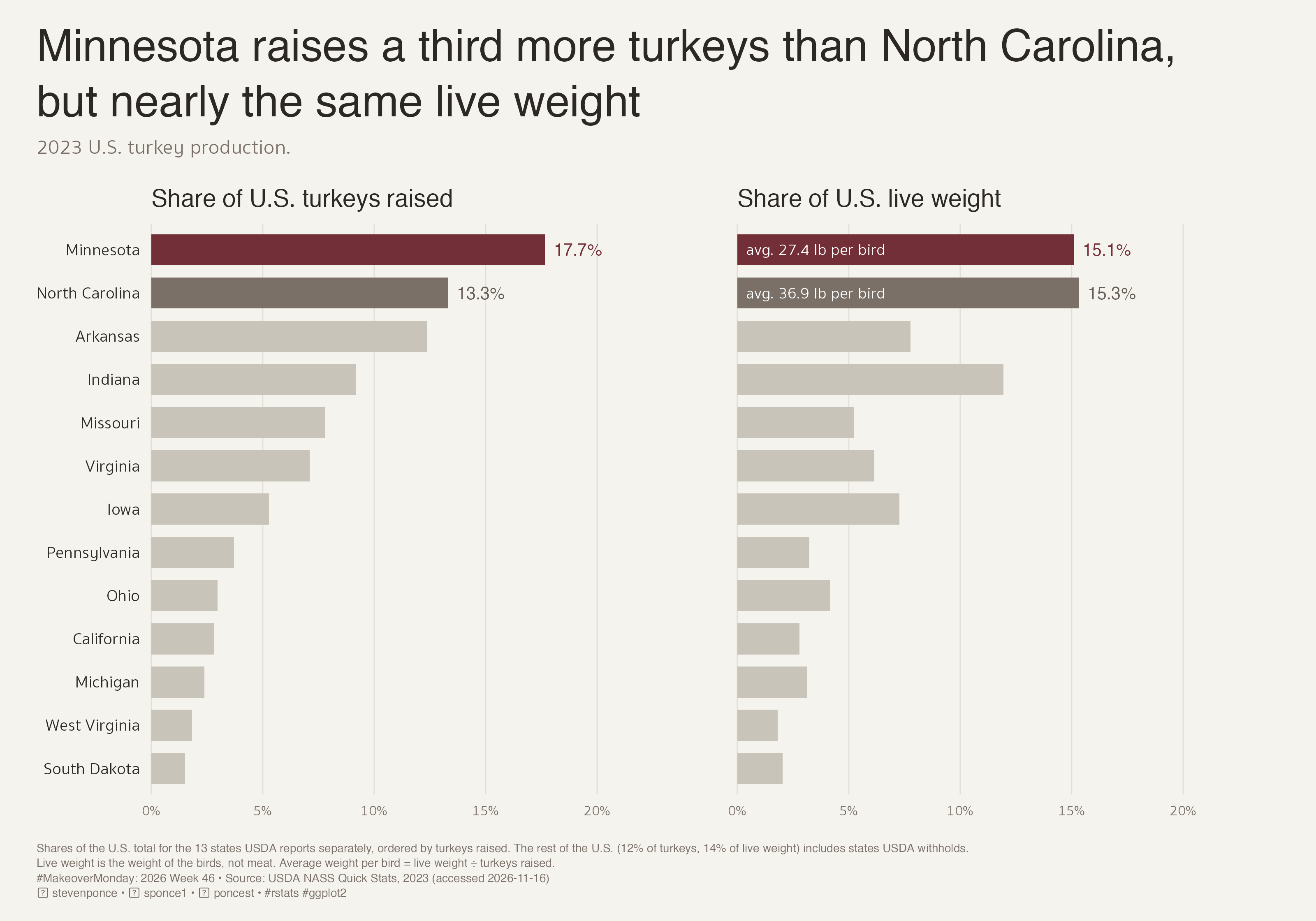
Minnesota raised a third more turkeys than North Carolina in 2023 (38.5 million vs 29.0 million), yet the two states produced nearly the same live weight: 1.05 vs 1.07 billion pounds. Shares of U.S. birds raised and of U.S. live weight are compared on one scale using USDA NASS data. Built in R with ggplot2 and rnassqs.
Author

Steven Ponce

Published

November 17, 2026

Original

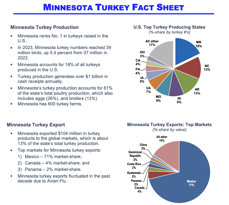
The original visualization comes from Minnesota Turkey Fact Sheet (MDA).

Original visualization

Makeover

Figure 1: Two side-by-side bar charts of 2023 U.S. turkey production for the 13 states, as reported separately by the USDA, sorted by turkeys raised, both on a 0–20% scale. The left panel shows share of U.S. turkeys raised: Minnesota led with 17.7%, well ahead of North Carolina at 13.3%. The right panel shows share of U.S. live weight: the two states were nearly equal, with Minnesota at 15.1% and North Carolina at 15.3%, because North Carolina’s birds averaged 36.9 lb compared with Minnesota’s 27.4 lb. Minnesota is highlighted in burgundy, North Carolina in warm gray, and the other 11 states in light gray; Indiana rises to the third-largest share by live weight. The remaining states, including those USDA withholds, account for 12% of turkeys and 14% of live weight. Source: USDA NASS Quick Stats, 2023.

Key takeaways

  • Minnesota’s “No. 1” ranking depends on what is measured. It leads in birds raised, but produces nearly the same total live weight as North Carolina.
  • North Carolina’s higher average live weight per bird (36.9 lb vs. 27.4 lb) almost exactly offsets Minnesota’s larger bird count.
  • Live weight is not meat production. States not reported separately account for 12% of U.S. turkeys and 14% of live weight, limiting comparisons beyond the top two.

Steps to Create this Graphic

1. Load Packages & Setup

Show code
```{r}
#| label: load
#| warning: false
#| message: false      
#| results: "hide"     

## 1. LOAD PACKAGES & SETUP ----
suppressPackageStartupMessages({
  if (!require("pacman")) install.packages("pacman")
  pacman::p_load(
    tidyverse, ggtext, showtext, scales, glue,
  ggview, readxl, magick, janitor, rnassqs
)
})

# Source utility functions
suppressMessages(
  source(here::here("R/utils/fonts.R")))
  source(here::here("R/utils/social_icons.R"))
  source(here::here("R/themes/base_theme.R"))

### |- figure size ----
fig_w <- 10
fig_h <- 7
fig_dpi <- 320

### |-  fonts ----
setup_fonts()
fonts <- get_font_families()
title_family <- fonts$title_1
text_family <- fonts$text
cap_family <- fonts$caption
```

2. Read in the Data

Show code
```{r}
#| label: read
#| include: true
#| eval: true
#| warning: false

xl_path <- here::here("data/MakeoverMonday/2026/minnesota_turkey_fact_sheet.xlsx")

states_raw <- read_excel(
  xl_path, sheet = "US Top Producing States", range = "A4:D15",
  col_types = c("text", "text", "text", "numeric")
) |> clean_names()

### |- USDA NASS 2023 (cached) ----
nass_path <- here::here("data/MakeoverMonday/2026/nass_turkeys_2023.rds")

if (!file.exists(nass_path)) {
  nass_pull <- rnassqs::nassqs(list(
    source_desc    = "SURVEY",
    commodity_desc = "TURKEYS",
    year           = 2023,
    agg_level_desc = c("STATE", "NATIONAL"),
    freq_desc      = "ANNUAL"
  ))
  saveRDS(nass_pull, nass_path)
}
nass_raw <- readRDS(nass_path) |> as_tibble()
```

3. Examine the Data

Show code
```{r}
#| label: examine
#| include: true
#| eval: true
#| results: 'hide'
#| warning: false

glimpse(states_raw)
nass_raw |> count(short_desc, unit_desc, reference_period_desc)
```

4. Tidy Data

Show code
```{r}
#| label: tidy
#| warning: false

### |- NASS: turkeys raised (head) and live-weight production (lb) ----
nass_items <- c(
  HEAD = "TURKEYS - PRODUCTION, MEASURED IN HEAD",
  LB   = "TURKEYS - PRODUCTION, MEASURED IN LB"
)

nass_wide <- nass_raw |>
  filter(short_desc %in% nass_items, reference_period_desc == "YEAR") |>
  mutate(unit = names(nass_items)[match(short_desc, nass_items)]) |>
  select(agg_level_desc, state_name, state_alpha, unit, value = Value) |>
  pivot_wider(names_from = unit, values_from = value) |>
  rename(head = HEAD, lb = LB)

us_tot <- filter(nass_wide, agg_level_desc == "NATIONAL")

states_nass <- nass_wide |>
  filter(agg_level_desc == "STATE", state_alpha != "OT") |> # OT = "Other States"
  mutate(
    lb_per_bird = lb / head,
    share_head  = head / us_tot$head,
    share_lb    = lb / us_tot$lb
  )

### |- residual: "Other States" (includes states NASS withholds) ----
nass_residual <- tibble(
  share_head = 1 - sum(states_nass$share_head),
  share_lb   = 1 - sum(states_nass$share_lb)
)

### |- plot data: one row per state x measure, one shared state order ----
measure_labels <- c(
  share_head = "Share of U.S. turkeys raised",
  share_lb   = "Share of U.S. live weight"
)

state_levels <- states_nass |>
  arrange(head) |>
  pull(state_name) |>
  str_to_title()

plot_df <- states_nass |>
  mutate(
    focus = case_when(state_alpha == "MN" ~ "MN", state_alpha == "NC" ~ "NC", .default = "other"),
    state = factor(str_to_title(state_name), levels = state_levels)
  ) |>
  select(state, state_alpha, focus, lb_per_bird, share_head, share_lb) |>
  pivot_longer(c(share_head, share_lb), names_to = "measure", values_to = "share") |>
  mutate(measure = factor(measure_labels[measure], levels = measure_labels))

pct1 <- label_percent(accuracy = 0.1)
pct0 <- label_percent(accuracy = 1)

label_df <- plot_df |>
  filter(focus != "other") |>
  mutate(label = pct1(share))

weight_df <- plot_df |>
  filter(focus != "other", measure == measure_labels[["share_lb"]]) |>
  mutate(label = glue("avg. {number(lb_per_bird, accuracy = 0.1)} lb per bird"))
```

5. Visualization Parameters

Show code
```{r}
#| label: params
#| include: true
#| warning: false

### |- plot aesthetics ----
colors <- get_theme_colors(
  palette = list(
    mn      = "#722F37",
    nc      = "#7A7068",
    nc_text = "#655C55",
    context = "#C9C4BA",
    ink     = "#2C2825",
    muted   = "#7A7068",
    grid    = "#E4DFD6"
  )
)
clrs <- colors$palette
col_mn <- clrs$mn
col_nc <- clrs$nc
col_nc_text <- clrs$nc_text
col_context <- clrs$context
col_ink <- clrs$ink
col_muted <- clrs$muted
col_grid <- clrs$grid

### |- titles and caption ----
# plain text: gridtext (textbox and markdown alike) widens word gaps with these fonts
title_text <- "Minnesota raises a third more turkeys than North Carolina,\nbut nearly the same live weight"

subtitle_text <- "2023 U.S. turkey production."

note_text <- glue(
  "Shares of the U.S. total for the 13 states USDA reports separately, ordered by turkeys raised. ",
  "The rest of the U.S. ({pct0(nass_residual$share_head)} of turkeys, ",
  "{pct0(nass_residual$share_lb)} of live weight) includes states USDA withholds.<br>",
  "Live weight is the weight of the birds, not meat. Average weight per bird = live weight ÷ turkeys raised."
)

caption_text <- paste0(
  note_text, "<br>",
  create_mm_caption(
    mm_year = 2026,
    mm_week = 46,
    source_text = "USDA NASS Quick Stats, 2023 (accessed 2026-11-16)"
  )
)

### |- plot theme ----
base_theme <- create_base_theme(colors)

weekly_theme <- extend_weekly_theme(
  base_theme,
  theme(
    panel.grid.major.y = element_blank(),
    panel.grid.minor = element_blank(),
    panel.grid.major.x = element_line(colour = col_grid, linewidth = 0.3),
    axis.ticks = element_blank(),
    axis.title = element_blank(),
    axis.text.y = element_text(family = text_family, size = rel(0.82), colour = col_ink, hjust = 1),
    axis.text.x = element_text(family = text_family, size = rel(0.70), colour = col_muted),
    strip.text = element_text(
      family = text_family, face = "bold", size = rel(0.95),
      colour = col_ink, hjust = 0, margin = margin(b = 8)
    ),
    panel.spacing.x = unit(28, "pt"),
    legend.position = "none",
    plot.title = element_text(
      family = title_family, size = rel(1.72), colour = col_ink,
      lineheight = 1.05, margin = margin(b = 8)
    ),
    plot.subtitle = element_text(
      family = text_family, size = rel(0.80), colour = col_muted,
      lineheight = 1.3, margin = margin(b = 16)
    ),
    plot.caption = element_textbox_simple(
      family = cap_family, size = rel(0.45), colour = col_muted,
      lineheight = 1.3, margin = margin(t = 14), width = unit(1, "npc")
    ),
    plot.margin = margin(16, 24, 12, 20)
  )
)

theme_set(weekly_theme)
```

6. Plot

Show code
```{r}
#| label: plot
#| warning: false

### |- main plot ----
p <- ggplot(plot_df, aes(x = share, y = state)) +
  geom_col(aes(fill = focus), width = 0.72) +
  geom_text(
    data = label_df,
    aes(label = label, colour = focus),
    hjust = 0, nudge_x = 0.004,
    family = text_family, fontface = "bold", size = 3.3
  ) +
  geom_text(
    data = weight_df,
    aes(label = label),
    x = 0.004, hjust = 0, colour = "white",
    family = text_family, size = 3.1
  ) +
  scale_fill_manual(values = c(MN = col_mn, NC = col_nc, other = col_context)) +
  scale_colour_manual(values = c(MN = col_mn, NC = col_nc_text)) +
  scale_x_continuous(
    limits = c(0, 0.20), breaks = seq(0, 0.20, 0.05),
    labels = label_percent(), expand = expansion(mult = c(0, 0.20))
  ) +
  scale_y_discrete(limits = state_levels) +
  coord_cartesian(clip = "off") +
  facet_wrap(~measure, nrow = 1) +
  labs(title = title_text, subtitle = subtitle_text, caption = caption_text)
```

7. Save

Show code
```{r}
#| label: save
#| warning: false

### |- save ----
main_path  <- here::here("data_visualizations", "MakeoverMonday", "2026", "mm_2026_46.png")
thumb_path <- here::here("data_visualizations", "MakeoverMonday", "2026", "thumbnails", "mm_2026_46.png")

# Full-size version, for the QMD figure
save_ggplot(
  plot = p,
  file = main_path,
  width = fig_w, height = fig_h,
  units = "in", dpi = 320,
)

# Reduced-size thumbnail
fs::dir_create(dirname(thumb_path))
magick::image_read(main_path) |>
  magick::image_resize("400") |>
  magick::image_write(thumb_path)
```

8. Session Info

TipExpand for Session Info
R version 4.6.1 (2026-06-24)
Platform: aarch64-apple-darwin23
Running under: macOS Tahoe 26.7.3

Matrix products: default
BLAS:   /Library/Frameworks/R.framework/Versions/4.6/Resources/lib/libRblas.0.dylib 
LAPACK: /Library/Frameworks/R.framework/Versions/4.6/Resources/lib/libRlapack.dylib;  LAPACK version 3.12.1

locale:
[1] en_US.UTF-8/en_US.UTF-8/en_US.UTF-8/C/en_US.UTF-8/en_US.UTF-8

time zone: America/New_York
tzcode source: internal

attached base packages:
[1] stats     graphics  grDevices utils     datasets  methods   base     

other attached packages:
 [1] here_1.0.2      rnassqs_0.6.3   janitor_2.2.1   magick_2.9.1   
 [5] readxl_1.5.0    ggview_0.2.2    glue_1.8.1      scales_1.4.0   
 [9] showtext_0.9-8  showtextdb_3.0  sysfonts_0.8.9  ggtext_0.2.0   
[13] lubridate_1.9.5 forcats_1.0.1   stringr_1.6.0   dplyr_1.2.1    
[17] purrr_1.2.2     readr_2.2.0     tidyr_1.3.2     tibble_3.3.1   
[21] ggplot2_4.0.3   tidyverse_2.0.0 pacman_0.5.1   

loaded via a namespace (and not attached):
 [1] gtable_0.3.6       xfun_0.60          htmlwidgets_1.6.4  tzdb_0.5.0        
 [5] vctrs_0.7.3        tools_4.6.1        generics_0.1.4     pkgconfig_2.0.3   
 [9] RColorBrewer_1.1-3 S7_0.2.2           rematch_2.0.0      lifecycle_1.0.5   
[13] compiler_4.6.1     farver_2.1.2       textshaping_1.0.5  codetools_0.2-20  
[17] snakecase_0.11.1   litedown_0.10      htmltools_0.5.9    yaml_2.3.12       
[21] pillar_1.11.1      commonmark_2.0.0   tidyselect_1.2.1   digest_0.6.39     
[25] stringi_1.8.7      rprojroot_2.1.1    fastmap_1.2.0      grid_4.6.1        
[29] cli_3.6.6          magrittr_2.0.5     utf8_1.2.6         withr_3.0.3       
[33] timechange_0.4.0   rmarkdown_2.31     otel_0.2.0         cellranger_1.1.0  
[37] ragg_1.5.2         hms_1.1.4          evaluate_1.0.5     knitr_1.51        
[41] markdown_2.0       rlang_1.3.0        gridtext_0.1.6     Rcpp_1.1.2        
[45] xml2_1.6.0         rstudioapi_0.19.0  jsonlite_2.0.0     R6_2.6.1          
[49] fs_2.1.0           systemfonts_1.3.2 

9. GitHub Repository

TipExpand for GitHub Repo

The complete code for this analysis is available in mm_2026_46.qmd.

For the full repository, click here.

10. References

TipExpand for References

Primary Data (Makeover Monday): 1. Makeover Monday 2026 Week 46: Minnesota Turkey Fact Sheet - Workbook: three sheets retyping the fact sheet’s own figures (9 key metrics plus a 3-row poultry split; 11 producing-state shares including “All other”; 8 export markets). - The state shares sum to 101%. North Carolina and Arkansas are shown tied at 13%, but NASS has them at 13.3% and 12.4%, so the tie comes from rounding. - California is shown at 4%, but NASS has it at 2.8%, below Ohio. It is the only slice that doesn’t reconcile within 0.6 percentage points, so the pie’s figures are not used.

Source Data: 2. Minnesota Department of Agriculture (Su Ye). Minnesota Turkey Fact Sheet (2023). Sources listed: USDA, MDA, Minnesota Turkey Growers Association, FAO. - The 39 million birds is NASS’s September 2023 forecast; the final 2023 figure is 38.5 million. - “Over $1 billion” in cash receipts matches 2022’s production value ($1,044 million); 2023’s was $991.6 million (NASS Poultry Production and Value 2023 Summary, April 2024). - The $104 million in exports is about 10.5% of 2023 production value, not the stated 13%; the sheet doesn’t say what base it used.

Enrichment Data: 3. USDA National Agricultural Statistics Service. Quick Stats, accessed 2026-11-16 via rnassqs: TURKEYS - PRODUCTION, MEASURED IN HEAD and MEASURED IN LB, 2023, state and national. - 13 states plus “Other States” and the U.S. total. The parts sum exactly to the U.S. total: 218.0 million birds and 6,985,506,000 lb live weight. - The April 2024 summary had 6,985,916,000 lb. The 410,000 lb difference comes from NASS’s later Pennsylvania/California restatement; the bird total is unchanged. - Turkeys raised are estimated from a census of all known grow-out operations, so there is no sampling error. The risk is revision.

Original Visualization: 4. The fact sheet’s two pies: an 11-slice pie of U.S. producing states by number of birds, with Minnesota exploded, and a 9-slice pie of Minnesota export markets by value. Both pies repeat the figures in the adjacent text.

Prior Coverage: 5. WATTAgNet (2021). Top turkey producing states differ by head, weight. It reports that Minnesota leads by birds and North Carolina by pounds. This makeover re-reads the fact sheet with that distinction; the distinction itself is not new.

Analysis Frame: - Population: the 13 states USDA reports separately. “Other States” (12.1% of birds, 14.0% of live weight) includes states USDA withholds and appears only in the caption. - Measures: share of U.S. turkeys raised (head) and share of U.S. live weight (lb), on one shared 0–20% axis. Live weight is the weight of the birds, not meat. Average weight per bird = live weight ÷ turkeys raised. - Minnesota: 38.5 million birds (17.7%), 1,054.9 million lb (15.1%), 27.4 lb per bird. - North Carolina: 29.0 million birds (13.3%), 1,070.1 million lb (15.3%), 36.9 lb per bird. - Gaps: Minnesota raised 9.5 million more birds, about a third more. North Carolina produced 15.2 million lb more, 1.4% of its total, which the chart calls “nearly the same”. North Carolina is never named No. 1. - Claim limits: no withheld state can reach second place on either measure (“Other States” totals 26.3 million birds against 29.0 million, and 980.7 million lb against 1,054.9 million). Ranks below the top two hold only among the published states. - Not used: value of production, because NASS computes it as pounds times one national price, so it adds nothing beyond live weight; and exports, because Mexico’s 71% share is the fact sheet’s own headline and doesn’t bear on birds versus weight. - Scope: descriptive. State averages mix hens and toms, so the chart makes no claim about why the birds differ in weight.

11. Custom Functions Documentation

Note📦 Custom Helper Functions

This analysis uses custom functions from my personal module library for efficiency and consistency across projects.

Functions Used:

  • fonts.R: setup_fonts(), get_font_families() - Font management with showtext
  • social_icons.R: create_social_caption() - Generates formatted social media captions
  • base_theme.R: create_base_theme(), extend_weekly_theme(), get_theme_colors() - Custom ggplot2 themes

Why custom functions?
These utilities standardize theming, fonts, and output across all my data visualizations. The core analysis (data tidying and visualization logic) uses only standard tidyverse packages.

Source Code:
View all custom functions → GitHub: R/utils

Back to top

Citation

BibTeX citation:
@online{ponce2026,
  author = {Ponce, Steven},
  title = {Minnesota Raises a Third More Turkeys Than {North}
    {Carolina,} but Nearly the Same Live Weight},
  date = {2026-11-17},
  url = {https://stevenponce.netlify.app/data_visualizations/MakeoverMonday/2026/mm_2026_46.html},
  langid = {en}
}
For attribution, please cite this work as:
Ponce, Steven. 2026. “Minnesota Raises a Third More Turkeys Than North Carolina, but Nearly the Same Live Weight.” November 17. https://stevenponce.netlify.app/data_visualizations/MakeoverMonday/2026/mm_2026_46.html.
Source Code
---
title: "Minnesota raises a third more turkeys than North Carolina, but nearly the same live weight"
subtitle: "2023 U.S. turkey production."
description: "Minnesota raised a third more turkeys than North Carolina in 2023 (38.5 million vs 29.0 million), yet the two states produced nearly the same live weight: 1.05 vs 1.07 billion pounds. Shares of U.S. birds raised and of U.S. live weight are compared on one scale using USDA NASS data. Built in R with ggplot2 and rnassqs."
date: "2026-11-17"
author:
  - name: "Steven Ponce"
    url: "https://stevenponce.netlify.app"
citation:
  url: "https://stevenponce.netlify.app/data_visualizations/MakeoverMonday/2026/mm_2026_46.html"
categories: ["MakeoverMonday", "2026"]
tags: [
  "makeover-monday",
  "bar-chart",
  "two-panel",
  "agriculture",
  "poultry",
  "turkey",
  "usda-nass",
  "rnassqs",
  "minnesota",
  "ranking",
  "normalization",
  "ggplot2",
  "2026"
]
image: "thumbnails/mm_2026_46.png"
format:
  html:
    toc: true
    toc-depth: 5
    code-link: true
    code-fold: true
    code-tools: true
    code-summary: "Show code"
editor_options: 
  chunk_output_type: inline
execute: 
  freeze: true
  cache: true
  error: false
  message: false
  warning: false
  eval: true
---

```{r}
#| label: setup-links
#| include: false

# CENTRALIZED LINK MANAGEMENT

## Weekly inputs (the only lines to edit) ----
current_year   <- 2026
current_week   <- 46
mm_slug        <- "mn-turkey-fact-sheet"
source_article <- "https://www.mda.state.mn.us/sites/default/files/inline-files/MN%20turkey%20fact%20sheet%20%282023%29.pdf"   # SOURCE ARTICLE on the MM page
data_source    <- "https://www.mda.state.mn.us/sites/default/files/inline-files/MN%20turkey%20fact%20sheet%20%282023%29.pdf"   # DATA SOURCE on the MM page

## Derived (don't edit) ----
project_id     <- sprintf("mm_%d_%02d", current_year, current_week)
project_file   <- paste0(project_id, ".qmd")
mm_page        <- paste0("https://makeovermonday.vercel.app/dataset/", mm_slug)
chart_original <- sprintf(
"https://raw.githubusercontent.com/poncest/MakeoverMonday/refs/heads/master/%d/Week_%02d/original_chart.png", current_year, current_week)
repo_main      <- "https://github.com/poncest/personal-website/"
repo_file      <- paste0(
  repo_main, "blob/master/data_visualizations/MakeoverMonday/",
  current_year, "/", project_file
)

## Helper ----
create_link <- function(text, url) paste0("[", text, "](", url, ")")
```

### Original

The original visualization comes from `r create_link("Minnesota Turkey Fact Sheet (MDA)", source_article)`.
![Original visualization](https://raw.githubusercontent.com/poncest/MakeoverMonday/refs/heads/master/2026/Week_46/original_chart.png)

### Makeover

![Two side-by-side bar charts of 2023 U.S. turkey production for the 13 states, as reported separately by the USDA, sorted by turkeys raised, both on a 0–20% scale. The left panel shows share of U.S. turkeys raised: Minnesota led with 17.7%, well ahead of North Carolina at 13.3%. The right panel shows share of U.S. live weight: the two states were nearly equal, with Minnesota at 15.1% and North Carolina at 15.3%, because North Carolina's birds averaged 36.9 lb compared with Minnesota's 27.4 lb. Minnesota is highlighted in burgundy, North Carolina in warm gray, and the other 11 states in light gray; Indiana rises to the third-largest share by live weight. The remaining states, including those USDA withholds, account for 12% of turkeys and 14% of live weight. Source: USDA NASS Quick Stats, 2023.](mm_2026_46.png){#fig-1}

::: {.key-takeaways}
[Key takeaways]{.key-takeaways-label}

- Minnesota's "No. 1" ranking depends on what is measured. 
  It leads in birds raised, but produces nearly the same 
  total live weight as North Carolina.
- North Carolina's higher average live weight per bird 
  (36.9 lb vs. 27.4 lb) almost exactly offsets Minnesota's 
  larger bird count.
- Live weight is not meat production. States not reported 
  separately account for 12% of U.S. turkeys and 14% of 
  live weight, limiting comparisons beyond the top two.
:::

### [**Steps to Create this Graphic**]{.mark}

#### [1. Load Packages & Setup]{.smallcaps}

```{r}
#| label: load
#| warning: false
#| message: false      
#| results: "hide"     

## 1. LOAD PACKAGES & SETUP ----
suppressPackageStartupMessages({
  if (!require("pacman")) install.packages("pacman")
  pacman::p_load(
    tidyverse, ggtext, showtext, scales, glue,
  ggview, readxl, magick, janitor, rnassqs
)
})

# Source utility functions
suppressMessages(
  source(here::here("R/utils/fonts.R")))
  source(here::here("R/utils/social_icons.R"))
  source(here::here("R/themes/base_theme.R"))

### |- figure size ----
fig_w <- 10
fig_h <- 7
fig_dpi <- 320

### |-  fonts ----
setup_fonts()
fonts <- get_font_families()
title_family <- fonts$title_1
text_family <- fonts$text
cap_family <- fonts$caption
```

#### [2. Read in the Data]{.smallcaps}

```{r}
#| label: read
#| include: true
#| eval: true
#| warning: false

xl_path <- here::here("data/MakeoverMonday/2026/minnesota_turkey_fact_sheet.xlsx")

states_raw <- read_excel(
  xl_path, sheet = "US Top Producing States", range = "A4:D15",
  col_types = c("text", "text", "text", "numeric")
) |> clean_names()

### |- USDA NASS 2023 (cached) ----
nass_path <- here::here("data/MakeoverMonday/2026/nass_turkeys_2023.rds")

if (!file.exists(nass_path)) {
  nass_pull <- rnassqs::nassqs(list(
    source_desc    = "SURVEY",
    commodity_desc = "TURKEYS",
    year           = 2023,
    agg_level_desc = c("STATE", "NATIONAL"),
    freq_desc      = "ANNUAL"
  ))
  saveRDS(nass_pull, nass_path)
}
nass_raw <- readRDS(nass_path) |> as_tibble()
```

#### [3. Examine the Data]{.smallcaps}

```{r}
#| label: examine
#| include: true
#| eval: true
#| results: 'hide'
#| warning: false

glimpse(states_raw)
nass_raw |> count(short_desc, unit_desc, reference_period_desc)
```

#### [4. Tidy Data]{.smallcaps}

```{r}
#| label: tidy
#| warning: false

### |- NASS: turkeys raised (head) and live-weight production (lb) ----
nass_items <- c(
  HEAD = "TURKEYS - PRODUCTION, MEASURED IN HEAD",
  LB   = "TURKEYS - PRODUCTION, MEASURED IN LB"
)

nass_wide <- nass_raw |>
  filter(short_desc %in% nass_items, reference_period_desc == "YEAR") |>
  mutate(unit = names(nass_items)[match(short_desc, nass_items)]) |>
  select(agg_level_desc, state_name, state_alpha, unit, value = Value) |>
  pivot_wider(names_from = unit, values_from = value) |>
  rename(head = HEAD, lb = LB)

us_tot <- filter(nass_wide, agg_level_desc == "NATIONAL")

states_nass <- nass_wide |>
  filter(agg_level_desc == "STATE", state_alpha != "OT") |> # OT = "Other States"
  mutate(
    lb_per_bird = lb / head,
    share_head  = head / us_tot$head,
    share_lb    = lb / us_tot$lb
  )

### |- residual: "Other States" (includes states NASS withholds) ----
nass_residual <- tibble(
  share_head = 1 - sum(states_nass$share_head),
  share_lb   = 1 - sum(states_nass$share_lb)
)

### |- plot data: one row per state x measure, one shared state order ----
measure_labels <- c(
  share_head = "Share of U.S. turkeys raised",
  share_lb   = "Share of U.S. live weight"
)

state_levels <- states_nass |>
  arrange(head) |>
  pull(state_name) |>
  str_to_title()

plot_df <- states_nass |>
  mutate(
    focus = case_when(state_alpha == "MN" ~ "MN", state_alpha == "NC" ~ "NC", .default = "other"),
    state = factor(str_to_title(state_name), levels = state_levels)
  ) |>
  select(state, state_alpha, focus, lb_per_bird, share_head, share_lb) |>
  pivot_longer(c(share_head, share_lb), names_to = "measure", values_to = "share") |>
  mutate(measure = factor(measure_labels[measure], levels = measure_labels))

pct1 <- label_percent(accuracy = 0.1)
pct0 <- label_percent(accuracy = 1)

label_df <- plot_df |>
  filter(focus != "other") |>
  mutate(label = pct1(share))

weight_df <- plot_df |>
  filter(focus != "other", measure == measure_labels[["share_lb"]]) |>
  mutate(label = glue("avg. {number(lb_per_bird, accuracy = 0.1)} lb per bird"))

```

#### [5. Visualization Parameters]{.smallcaps}

```{r}
#| label: params
#| include: true
#| warning: false

### |- plot aesthetics ----
colors <- get_theme_colors(
  palette = list(
    mn      = "#722F37",
    nc      = "#7A7068",
    nc_text = "#655C55",
    context = "#C9C4BA",
    ink     = "#2C2825",
    muted   = "#7A7068",
    grid    = "#E4DFD6"
  )
)
clrs <- colors$palette
col_mn <- clrs$mn
col_nc <- clrs$nc
col_nc_text <- clrs$nc_text
col_context <- clrs$context
col_ink <- clrs$ink
col_muted <- clrs$muted
col_grid <- clrs$grid

### |- titles and caption ----
# plain text: gridtext (textbox and markdown alike) widens word gaps with these fonts
title_text <- "Minnesota raises a third more turkeys than North Carolina,\nbut nearly the same live weight"

subtitle_text <- "2023 U.S. turkey production."

note_text <- glue(
  "Shares of the U.S. total for the 13 states USDA reports separately, ordered by turkeys raised. ",
  "The rest of the U.S. ({pct0(nass_residual$share_head)} of turkeys, ",
  "{pct0(nass_residual$share_lb)} of live weight) includes states USDA withholds.<br>",
  "Live weight is the weight of the birds, not meat. Average weight per bird = live weight ÷ turkeys raised."
)

caption_text <- paste0(
  note_text, "<br>",
  create_mm_caption(
    mm_year = 2026,
    mm_week = 46,
    source_text = "USDA NASS Quick Stats, 2023 (accessed 2026-11-16)"
  )
)

### |- plot theme ----
base_theme <- create_base_theme(colors)

weekly_theme <- extend_weekly_theme(
  base_theme,
  theme(
    panel.grid.major.y = element_blank(),
    panel.grid.minor = element_blank(),
    panel.grid.major.x = element_line(colour = col_grid, linewidth = 0.3),
    axis.ticks = element_blank(),
    axis.title = element_blank(),
    axis.text.y = element_text(family = text_family, size = rel(0.82), colour = col_ink, hjust = 1),
    axis.text.x = element_text(family = text_family, size = rel(0.70), colour = col_muted),
    strip.text = element_text(
      family = text_family, face = "bold", size = rel(0.95),
      colour = col_ink, hjust = 0, margin = margin(b = 8)
    ),
    panel.spacing.x = unit(28, "pt"),
    legend.position = "none",
    plot.title = element_text(
      family = title_family, size = rel(1.72), colour = col_ink,
      lineheight = 1.05, margin = margin(b = 8)
    ),
    plot.subtitle = element_text(
      family = text_family, size = rel(0.80), colour = col_muted,
      lineheight = 1.3, margin = margin(b = 16)
    ),
    plot.caption = element_textbox_simple(
      family = cap_family, size = rel(0.45), colour = col_muted,
      lineheight = 1.3, margin = margin(t = 14), width = unit(1, "npc")
    ),
    plot.margin = margin(16, 24, 12, 20)
  )
)

theme_set(weekly_theme)
```

#### [6. Plot]{.smallcaps}

```{r}
#| label: plot
#| warning: false

### |- main plot ----
p <- ggplot(plot_df, aes(x = share, y = state)) +
  geom_col(aes(fill = focus), width = 0.72) +
  geom_text(
    data = label_df,
    aes(label = label, colour = focus),
    hjust = 0, nudge_x = 0.004,
    family = text_family, fontface = "bold", size = 3.3
  ) +
  geom_text(
    data = weight_df,
    aes(label = label),
    x = 0.004, hjust = 0, colour = "white",
    family = text_family, size = 3.1
  ) +
  scale_fill_manual(values = c(MN = col_mn, NC = col_nc, other = col_context)) +
  scale_colour_manual(values = c(MN = col_mn, NC = col_nc_text)) +
  scale_x_continuous(
    limits = c(0, 0.20), breaks = seq(0, 0.20, 0.05),
    labels = label_percent(), expand = expansion(mult = c(0, 0.20))
  ) +
  scale_y_discrete(limits = state_levels) +
  coord_cartesian(clip = "off") +
  facet_wrap(~measure, nrow = 1) +
  labs(title = title_text, subtitle = subtitle_text, caption = caption_text)
```

#### [7. Save]{.smallcaps}

```{r}
#| label: save
#| warning: false

### |- save ----
main_path  <- here::here("data_visualizations", "MakeoverMonday", "2026", "mm_2026_46.png")
thumb_path <- here::here("data_visualizations", "MakeoverMonday", "2026", "thumbnails", "mm_2026_46.png")

# Full-size version, for the QMD figure
save_ggplot(
  plot = p,
  file = main_path,
  width = fig_w, height = fig_h,
  units = "in", dpi = 320,
)

# Reduced-size thumbnail
fs::dir_create(dirname(thumb_path))
magick::image_read(main_path) |>
  magick::image_resize("400") |>
  magick::image_write(thumb_path)
```

#### [8. Session Info]{.smallcaps}

::: {.callout-tip collapse="true"}
##### Expand for Session Info

```{r, echo = FALSE}
#| eval: true
#| warning: false

sessionInfo()
```
:::

#### [9. GitHub Repository]{.smallcaps}

::: {.callout-tip collapse="true"}
##### Expand for GitHub Repo

The complete code for this analysis is available in `r create_link(project_file, repo_file)`.

For the full repository, `r create_link("click here", repo_main)`.
:::

#### [10. References]{.smallcaps}

::: {.callout-tip collapse="true"}
##### Expand for References

**Primary Data (Makeover Monday):** 1.
Makeover Monday `r current_year` Week `r current_week`: `r create_link("Minnesota Turkey Fact Sheet", mm_page)` - Workbook: three sheets retyping the fact sheet's own figures (9 key metrics plus a 3-row poultry split; 11 producing-state shares including "All other"; 8 export markets).
- The state shares sum to 101%. North Carolina and Arkansas are shown tied at 13%, but NASS has them at 13.3% and 12.4%, so the tie comes from rounding.
- California is shown at 4%, but NASS has it at 2.8%, below Ohio. It is the only slice that doesn't reconcile within 0.6 percentage points, so the pie's figures are not used.

**Source Data:** 2.
Minnesota Department of Agriculture (Su Ye). `r create_link("Minnesota Turkey Fact Sheet (2023)", source_article)`. Sources listed: USDA, MDA, Minnesota Turkey Growers Association, FAO.
- The 39 million birds is NASS's September 2023 forecast; the final 2023 figure is 38.5 million.
- "Over $1 billion" in cash receipts matches 2022's production value ($1,044 million); 2023's was $991.6 million (NASS Poultry Production and Value 2023 Summary, April 2024).
- The $104 million in exports is about 10.5% of 2023 production value, not the stated 13%; the sheet doesn't say what base it used.

**Enrichment Data:** 3.
USDA National Agricultural Statistics Service. `r create_link("Quick Stats", "https://quickstats.nass.usda.gov/")`, accessed 2026-11-16 via `rnassqs`: TURKEYS - PRODUCTION, MEASURED IN HEAD and MEASURED IN LB, 2023, state and national.
- 13 states plus "Other States" and the U.S. total. The parts sum exactly to the U.S. total: 218.0 million birds and 6,985,506,000 lb live weight.
- The April 2024 summary had 6,985,916,000 lb. The 410,000 lb difference comes from NASS's later Pennsylvania/California restatement; the bird total is unchanged.
- Turkeys raised are estimated from a census of all known grow-out operations, so there is no sampling error. The risk is revision.

**Original Visualization:** 4.
The fact sheet's two pies: an 11-slice pie of U.S. producing states by number of birds, with Minnesota exploded, and a 9-slice pie of Minnesota export markets by value. Both pies repeat the figures in the adjacent text.

**Prior Coverage:** 5.
WATTAgNet (2021). `r create_link("Top turkey producing states differ by head, weight", "https://wattagnet.com/articles/45299-top-turkey-producing-states-differ-by-head-weight")`. It reports that Minnesota leads by birds and North Carolina by pounds. This makeover re-reads the fact sheet with that distinction; the distinction itself is not new.

**Analysis Frame:** - **Population:** the 13 states USDA reports separately. "Other States" (12.1% of birds, 14.0% of live weight) includes states USDA withholds and appears only in the caption.
- **Measures:** share of U.S. turkeys raised (head) and share of U.S. live weight (lb), on one shared 0–20% axis. Live weight is the weight of the birds, not meat. Average weight per bird = live weight ÷ turkeys raised.
- **Minnesota:** 38.5 million birds (17.7%), 1,054.9 million lb (15.1%), 27.4 lb per bird.
- **North Carolina:** 29.0 million birds (13.3%), 1,070.1 million lb (15.3%), 36.9 lb per bird.
- **Gaps:** Minnesota raised 9.5 million more birds, about a third more. North Carolina produced 15.2 million lb more, 1.4% of its total, which the chart calls "nearly the same". North Carolina is never named No. 1.
- **Claim limits:** no withheld state can reach second place on either measure ("Other States" totals 26.3 million birds against 29.0 million, and 980.7 million lb against 1,054.9 million). Ranks below the top two hold only among the published states.
- **Not used:** value of production, because NASS computes it as pounds times one national price, so it adds nothing beyond live weight; and exports, because Mexico's 71% share is the fact sheet's own headline and doesn't bear on birds versus weight.
- **Scope:** descriptive. State averages mix hens and toms, so the chart makes no claim about why the birds differ in weight.
:::

#### [11. Custom Functions Documentation]{.smallcaps}

::: {.callout-note collapse="true"}
##### 📦 Custom Helper Functions

This analysis uses custom functions from my personal module library for efficiency and consistency across projects.

**Functions Used:**

- **`fonts.R`**: `setup_fonts()`, `get_font_families()` - Font management with showtext
- **`social_icons.R`**: `create_social_caption()` - Generates formatted social media captions
- **`base_theme.R`**: `create_base_theme()`, `extend_weekly_theme()`, `get_theme_colors()` - Custom ggplot2 themes

**Why custom functions?**\
These utilities standardize theming, fonts, and output across all my data visualizations.
The core analysis (data tidying and visualization logic) uses only standard tidyverse packages.

**Source Code:**\
View all custom functions → [GitHub: R/utils](https://github.com/poncest/personal-website/tree/master/R)
:::

© 2024–2026 Steven Ponce · Built with R + Quarto

Source Issues
