---
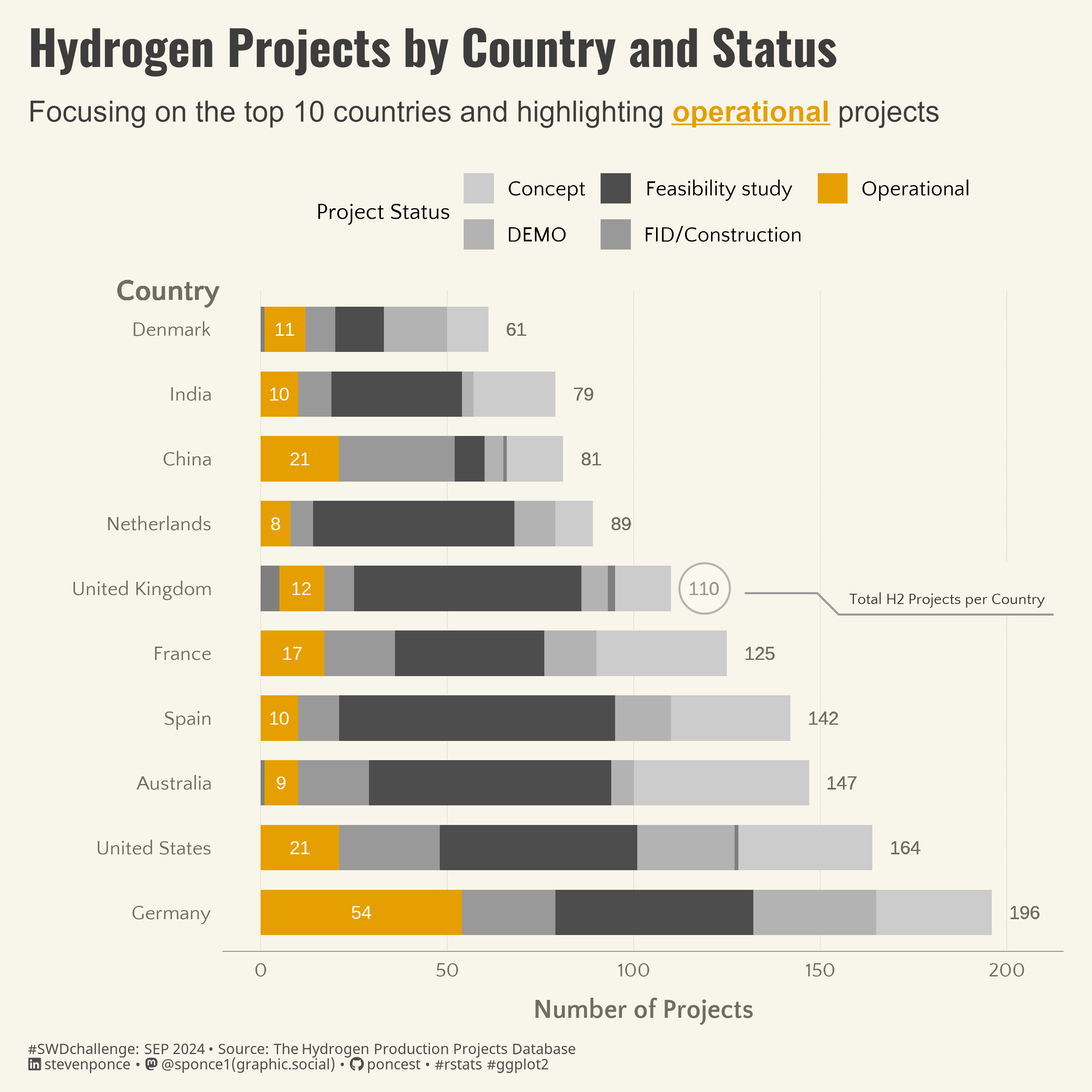
title: "Hydrogen Projects by Country and Status"
subtitle: "Focusing on the top 10 countries and highlighting operational projects"
author: "Steven Ponce"
description: "Hydrogen projects in the top 10 countries by status, with operational projects highlighted. Built in R."
date: "2024-09-01"
categories: ["SWDchallenge", "2024"]
image: "thumbnails/swd_2024_09.png"
format:
html:
toc: true
toc-depth: 5
code-link: true
code-fold: true
code-tools: true
editor_options:
chunk_output_type: console
execute:
freeze: true
error: false
message: false
warning: false
eval: false
# share:
# permalink: "https://stevenponce.netlify.app/data_visualizations.html"
# linkedin: true
# twitter: true
# email: true
---
{#fig-1}
### <mark> __Steps to Create this Graphic__ </mark>
#### 1. Load Packages & Setup
```{r}
#| label: load

pacman::p_load(
  tidyverse,   # Easily Install and Load the 'Tidyverse'
  ggtext,      # Improved Text Rendering Support for 'ggplot2'
  showtext,    # Using Fonts More Easily in R Graphs
  janitor,     # Simple Tools for Examining and Cleaning Dirty Data
  skimr,       # Compact and Flexible Summaries of Data
  scales,      # Scale Functions for Visualization
  lubridate,   # Make Dealing with Dates a Little Easier
  glue,        # Interpreted String Literals
  readxl,      # Read Excel Files
  countrycode, # Convert Country Names and Country Codes
  marquee,     # Markdown Parser and Renderer for R Graphics
  ggforce      # Accelerating 'ggplot2'
)

### |- figure size ----
camcorder::gg_record(
  dir    = here::here("temp_plots"),
  device = "png",
  width  = 8,
  height = 8,
  units  = "in",
  dpi    = 320)

### |- resolution ----
showtext_opts(dpi = 320, regular.wt = 300, bold.wt = 800)
```
#### 2. Read in the Data
```{r}
#| label: read

worldwide_hydrogen_projects <- read_xlsx(
  here::here("data/Hydrogen_production_projects_corrected.xlsx"),
  sheet = "Projects", skip = 3, trim_ws = TRUE
  ) |>
  clean_names() |>
  glimpse()
```
#### 3. Examine the Data
```{r}
#| label: examine

glimpse(worldwide_hydrogen_projects)
skim(worldwide_hydrogen_projects)
colnames(worldwide_hydrogen_projects)
```
#### 4. Tidy Data
```{r}
#| label: tidy

plot_data <- worldwide_hydrogen_projects |>
  filter(!is.na(country), !is.na(status)) |>
  count(country, status) |>
  # Lump less common countries into "Other"
  mutate(country = fct_lump(country, n = 10, w = n)) |>
  group_by(country) |>
  mutate(total_projects = sum(n)) |>
  ungroup() |>
  filter(country != "Other") |>
  # Convert ISO3 country codes to country names
  mutate(country = countrycode(country, origin = 'iso3c', destination = 'country.name')) |>
  arrange(desc(total_projects))
```
#### 5. Visualization Parameters
```{r}
#| label: params
### |- plot aesthetics ----
bkg_col <- colorspace::lighten('#f7f5e9', 0.05)
title_col <- "#3d3d3d"
subtitle_col <- "#3d3d3d"
caption_col <- "gray30"
text_col <- colorspace::darken("#8e8a7b" , 0.2)
# Define colors to highlight Operational projects
highlight_colors <- c(
"Operational" = "#E69F00", # Highlight color
"Concept" = "grey80",
"DEMO" = "grey70",
"FID/Construction" = "grey60",
"Other" = "grey50",
"Decomissioned" = "grey40",
"Feasibility study" = "grey30"
)
### |- titles and caption ----
# icons
tt <- str_glue("#SWDchallenge: SEP 2024 • Source: The Hydrogen Production Projects Database<br>")
li <- str_glue("<span style='font-family:fa6-brands'></span>")
gh <- str_glue("<span style='font-family:fa6-brands'></span>")
mn <- str_glue("<span style='font-family:fa6-brands'></span>")
# text
title_text <- str_glue("Hydrogen Projects by Country and Status")
subtitle_text <- "Focusing on the top 10 countries and highlighting {#E69F00 _**operational**_} projects"
caption_text <- str_glue("{tt} {li} stevenponce • {mn} @sponce1(graphic.social) • {gh} poncest • #rstats #ggplot2")
### |- fonts ----
font_add('fa6-brands', here::here('fonts/6.6.0/Font Awesome 6 Brands-Regular-400.otf'))
font_add_google("Oswald", regular.wt = 400, family = "title")
font_add_google("Quattrocento Sans", regular.wt = 400, family = "subtitle")
font_add_google("Quattrocento Sans", regular.wt = 400, family = "text")
font_add_google("Noto Sans", regular.wt = 400,family = "caption")
showtext_auto(enable = TRUE)
### |- plot theme ----
theme_set(theme_minimal(base_size = 14, base_family = "text"))
theme_update(
plot.title.position = "plot",
plot.caption.position = "plot",
legend.position = "top",
legend.title = element_text(size = rel(.85), hjust = 0.5),
legend.text = element_text(size = rel(0.8)),
plot.margin = margin(t = 10, r = 15, b = 0, l = 15),
plot.background = element_rect(fill = bkg_col, color = bkg_col),
panel.background = element_rect(fill = bkg_col, color = bkg_col),
axis.title.x = element_text(margin = margin(10, 0, 0, 0), size = rel(1),
color = text_col, family = 'text', face = 'bold'),
axis.title.y = element_text(margin = margin(0, 10, 0, 0), size = rel(1),
color = text_col, family = 'text', face = 'bold'),
axis.text = element_text(size = rel(0.75), color = text_col, family = 'text'),
axis.line.x = element_line(color = "#7F7F7F", linewidth = 0.2),
panel.grid.minor.y = element_blank(),
panel.grid.major.y = element_blank(),
panel.grid.minor.x = element_blank(),
panel.grid.major.x = element_line(linetype = "dotted", linewidth = 0.1, color = 'gray40'),
)
```
#### 6. Plot
```{r}
#| label: plot

### |-  initial plot ----
p <- plot_data |>
  ggplot(aes(x = reorder(country, -total_projects), y = n, fill = status)) +

  # Geoms
  geom_bar(stat = "identity", position = "stack", width = 0.7) +

  # Add total project labels at the end of each bar
  geom_text(aes(label = total_projects),
            y = plot_data$total_projects + 5,
            hjust = 0, color = text_col, size = 3.5) +

  # Add labels specifically for Operational projects
  geom_text(aes(label = ifelse(status == "Operational", n, "")),
            position = position_stack(vjust = 0.5), color = "white", size = 3.5) +

  # Add country label above Denmark
  geom_text(aes(label = "Country", x = "Denmark", y = 0),
            size = 5.5, color = text_col, family = "text", fontface = "bold",
            hjust = 1.4, vjust = -1.5) +

  # Scales
  scale_x_discrete() +
  scale_y_continuous(limits = c(0, 205)) +
  scale_fill_manual(
    values = highlight_colors,
    guide = guide_legend(nrow = 2)
    ) +
  coord_flip(clip = 'off') +

  # Labs
  labs(
    x = "",
    y = "Number of Projects",
    fill = "Project Status",
    title    = title_text,
    subtitle = subtitle_text,
    caption  = caption_text,
  ) +

  # Theme
  theme(

    plot.title    = element_text(
      size        = rel(1.8),
      family      = "title",
      face        = "bold",
      color       = title_col,
      lineheight  = 1.1,
      margin      = margin(t = 5, b = 5)
    ),
    plot.subtitle = element_marquee(
      size        = rel(1.1),
      family      = 'subtitle',
      color       = subtitle_col,
      lineheight  = 1.4,
      margin      = margin(t = 5, b = 1)
    ),
    plot.caption  = element_markdown(
      size        = rel(.55),
      family      = 'caption',
      color       = caption_col,
      lineheight  = 0.6,
      hjust       = 0,
      halign      = 0,
      margin      = margin(t = 10, b = 10)
    )
  )

### |-  annotated plot ----

# label data
label_data <- tibble(
  country = "United Kingdom",
  total_projects = 119
)

p <- p +
  ggforce::geom_mark_circle(
    data = label_data,
    aes(
      x = country,
      y = total_projects,
      label = "",
      description = "Total H2 Projects per Country",
      ),
    expand = 0.03,
    label.buffer = unit(-1, "lines"),
    color = "gray70",
    fill = "transparent",
    label.fill = bkg_col,
    label.fontsize = 8,
    label.family = "text",
    con.type = "elbow",
    label.colour = 'gray20',
    con.colour = 'gray60'
  )
```
#### 7. Save
```{r}
#| label: save

### |-  plot image ----
ggsave(
  filename = here::here("data_visualizations/SWD Challenge/2024/swd_2024_09.png"),
  plot = p,
  width  =  8,
  height =  8,
  units  = "in",
  dpi    = 320
)

### |-  plot thumbnail----
magick::image_read(here::here("data_visualizations/SWD Challenge/2024/swd_2024_09.png")) |>
  magick::image_resize(geometry = "400") |>
  magick::image_write(here::here("data_visualizations/SWD Challenge/2024/thumbnails/swd_2024_09.png"))
```
#### 8. Session Info
::: {.callout-tip collapse="true"}
##### Expand for Session Info
```{r, echo = FALSE}
#| eval: true
sessionInfo()
```
:::
#### 9. GitHub Repository
::: {.callout-tip collapse="true"}
##### Expand for GitHub Repo
[Access the GitHub repository here](https://github.com/poncest/personal-website/)
:::
