---
title: "Summer delays arrive right on schedule"
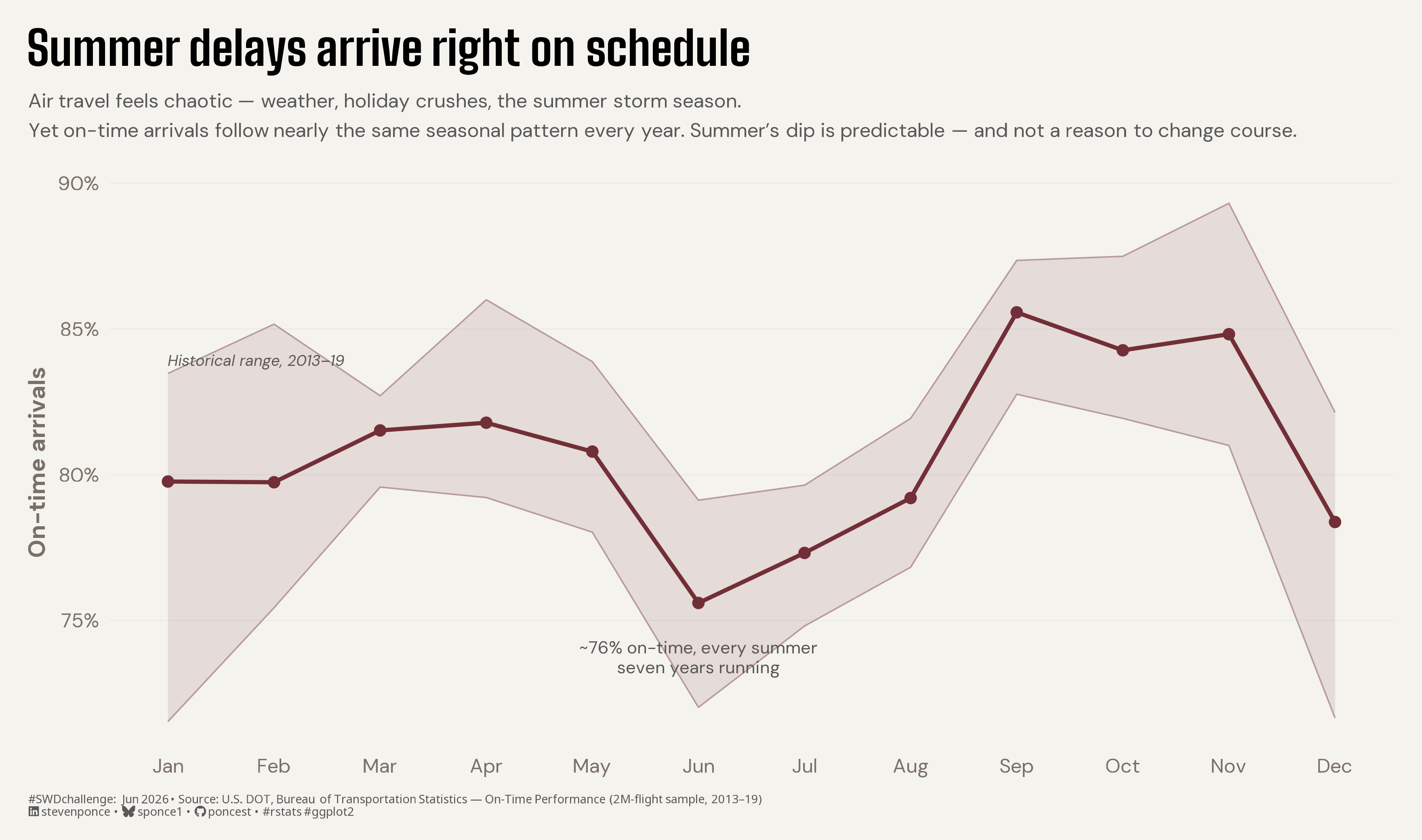
subtitle: "Air travel feels chaotic — weather, holiday crushes, the summer storm season. Yet on-time arrivals follow nearly the same seasonal pattern every year. Summer's dip is predictable — and not a reason to change course."
description: "U.S. airline on-time arrivals trace nearly the same seasonal path every year, so the summer dip reads as expected rather than alarming. A typical-year line (the 2013–2019 average) sits inside a band of the full historical range, framing the variation as containment, not a target to beat. Built in R with ggplot2, ggtext, and camcorder."
date: "2026-06-01"
author:
- name: "Steven Ponce"
url: "https://stevenponce.netlify.app"
citation:
url: "https://stevenponce.netlify.app/data_visualizations/SWD%20Challenge/2026/swd_2026_06.html"
categories: ["SWDchallenge", "2026"]
tags: [
"swd-challenge",
"line-chart",
"range-band",
"seasonality",
"airlines",
"on-time-performance",
"containment",
"stability",
"annotation",
"ggtext",
"camcorder",
"2026"
]
image: "thumbnails/swd_2026_06.png"
format:
html:
toc: true
toc-depth: 5
code-link: true
code-fold: true
code-tools: true
code-summary: "Show code"
editor_options:
chunk_output_type: inline
execute:
freeze: true
cache: true
error: false
message: false
warning: false
eval: true
---
### Challenge
Some stories are meaningful because of what hasn’t changed. This month, we challenge you to design a view in which the most important takeaway is that things are performing as expected and the best decision is to stay the course. Think beyond a general metrics update and focus on situations where highlighting what’s expected helps to inform a specific action.
Additional information can be found [HERE](https://community.storytellingwithdata.com/challenges)
### Visualization
{#fig-1}
### [**Steps to Create this Graphic**]{.mark}
#### [1. Load Packages & Setup]{.smallcaps}
```{r}
#| label: load

if (!require("pacman")) install.packages("pacman")
pacman::p_load(
  tidyverse, ggtext, showtext, janitor, scales, glue
)

### |- figure size ----
camcorder::gg_record(
  dir    = here::here("temp_plots"),
  device = "png",
  width  = 11,
  height = 6.5,
  units  = "in",
  dpi    = 320
)

# Source utility functions
suppressMessages(source(here::here("R/utils/fonts.R")))
source(here::here("R/utils/social_icons.R"))
source(here::here("R/utils/image_utils.R"))
source(here::here("R/themes/base_theme.R"))
```
#### [2. Read in the Data]{.smallcaps}
```{r}
#| label: read

raw_data <- read_csv(
  here::here("data/SWDchallenge/2026/airline_2m.csv"),
  show_col_types = FALSE
) |> clean_names()
```
#### [3. Examine the Data]{.smallcaps}
```{r}
#| label: examine
#| include: true
#| eval: true
#| results: 'hide'
#| warning: false

glimpse(raw_data)
```
#### [4. Tidy Data]{.smallcaps}
```{r}
#| label: tidy
#| output: false

monthly <- raw_data |>
  filter(year >= 2013, year <= 2019) |>
  transmute(year, month, operated = cancelled == 0, on_time = arr_del15 == 0) |>
  summarise(ontime_rate = mean(on_time[operated], na.rm = TRUE), .by = c(year, month)) |>
  arrange(year, month)

band_all <- monthly |> summarise(lo = min(ontime_rate), hi = max(ontime_rate), .by = month)
avg_path <- monthly |> summarise(ontime_rate = mean(ontime_rate), .by = month)

### |-  anchor coordinates ----
jun_y <- avg_path$ontime_rate[avg_path$month == 6]
```
#### [5. Visualization Parameters]{.smallcaps}
```{r}
#| label: params

### |-  plot aesthetics ----
clrs <- get_theme_colors(
  palette = list(
    band = "#722F37",
    edge = "#B89AA0",
    line = "#722F37",
    anno = "gray35",
    sub = "gray35"
  )
)

col_band <- clrs$palette$band
col_edge <- clrs$palette$edge
col_line <- clrs$palette$line
col_anno <- clrs$palette$anno
col_sub  <- clrs$palette$sub

### |- titles and caption ----
title_text <- "Summer delays arrive right on schedule"

subtitle_text <- glue(
  "Air travel feels chaotic \u2014 weather, holiday crushes, the summer storm season.<br>",
  "Yet on-time arrivals follow nearly the same seasonal pattern every year. ",
  "Summer's dip is predictable \u2014 and not a reason to change course."
)

caption_text <- create_swd_caption(
  year = 2026, month = "Jun",
  source_text = "U.S. DOT, Bureau of Transportation Statistics \u2014 On-Time Performance (2M-flight sample, 2013\u201319)"
)

### |-  fonts ----
setup_fonts()
fonts <- get_font_families()

### |-  plot theme ----
base_theme <- create_base_theme(clrs)

weekly_theme <- extend_weekly_theme(
  base_theme,
  theme(
    panel.grid.minor = element_blank(),
    panel.grid.major.x = element_blank(),
    panel.grid.major.y = element_line(color = "gray92", linewidth = 0.3),
    axis.ticks = element_blank(),
    plot.title.position = "plot",
    plot.caption = element_markdown(hjust = 0)
  )
)

theme_set(weekly_theme)
```
#### [6. Plot]{.smallcaps}
```{r}
#| label: plot
#| output: false

### |- main plot ----
p <- ggplot() +
  # Geoms
  geom_ribbon(
    data = band_all, aes(month, ymin = lo, ymax = hi),
    fill = col_band, alpha = 0.12
  ) +
  geom_line(data = band_all, aes(month, lo), color = col_edge, linewidth = 0.4) +
  geom_line(data = band_all, aes(month, hi), color = col_edge, linewidth = 0.4) +
  geom_line(data = avg_path, aes(month, ontime_rate), color = col_line, linewidth = 1.1) +
  geom_point(data = avg_path, aes(month, ontime_rate), color = col_line, size = 2.4) +
  # Annotate
  annotate("text",
    x = 6, y = jun_y, vjust = 2.2, hjust = 0.5,
    family = fonts$text, size = 3.4, lineheight = 0.95, color = col_anno,
    label = "~76% on-time, every summer\nseven years running"
  ) +
  annotate("text",
    x = 1, y = band_all$hi[band_all$month == 1], hjust = 0, vjust = -0.7,
    family = fonts$text, size = 3, fontface = "italic", color = col_anno,
    label = "Historical range, 2013\u201319"
  ) +
  # Scales
  scale_x_continuous(breaks = 1:12, labels = month.abb) +
  scale_y_continuous(labels = label_percent(accuracy = 1)) +
  # Labs
  labs(
    title = title_text, subtitle = subtitle_text,
    x = NULL, y = "On-time arrivals", caption = caption_text
  ) +
  coord_cartesian(clip = "off") +
  # Theme
  theme(
    plot.title = element_markdown(
      size = 26, face = "bold", family = fonts$title_1,
      color = clrs$palette$title, margin = margin(b = 10), lineheight = 1.2
    ),
    plot.subtitle = element_textbox_simple(
      size = 11, family = fonts$text, color = col_sub,
      lineheight = 1.5, margin = margin(b = 20)
    ),
    plot.caption = element_markdown(
      size = 6.5, family = fonts$caption, color = col_sub,
      hjust = 0, margin = margin(t = 10)
    ),
    plot.background = element_rect(fill = clrs$palette$bg, color = NA),
    plot.margin = margin(16, 16, 12, 16)
  )
```
#### [7. Save]{.smallcaps}
```{r}
#| label: save

### |-  plot image ----
save_plot(
  p,
  type = 'swd',
  year = 2026,
  month = 06,
  width  = 11,
  height = 6.5,
  )
```
#### [8. Session Info]{.smallcaps}
::: {.callout-tip collapse="true"}
##### Expand for Session Info
```{r, echo = FALSE}
#| eval: true
#| warning: false
sessionInfo()
```
:::
#### [9. GitHub Repository]{.smallcaps}
::: {.callout-tip collapse="true"}
##### Expand for GitHub Repo
The complete code for this analysis is available in [`swd_2026_06.qmd`](https://github.com/poncest/personal-website/tree/master/data_visualizations/SWD%20Challenge/2026/swd_2026_06.qmd). For the full repository, [click here](https://github.com/poncest/personal-website/).
:::
#### [10. References]{.smallcaps}
::: {.callout-tip collapse="true"}
##### Expand for References
**SWD Challenge:**
- Storytelling with Data: [June 2026 — when normal is noteworthy](https://community.storytellingwithdata.com/challenges/jun-2026-when-normal-is-noteworthy)
**Data Sources:**
- Bureau of Transportation Statistics. *Reporting Carrier On-Time Performance*. U.S. Department of Transportation. <https://www.transtats.bts.gov/>
- mexwell. *Carrier On-Time Performance Dataset*. Kaggle. <https://www.kaggle.com/datasets/mexwell/carrier-on-time-performance-dataset> — a ~2M-flight random sample of the BTS data; full years 2013–2019 analyzed.
**Background References:**
- U.S. Department of Transportation. *Air Travel Consumer Report*. <https://www.transportation.gov/airconsumer> — national on-time arrival rate, ~79–80% across 2013–2019 (79.0% for full-year 2019), used as the reference average.
**Book Reference:**
- Knaflic, C. N. (2015). *Storytelling with Data: A Data Visualization Guide for Business Professionals*. Wiley.
:::
#### [11. Custom Functions Documentation]{.smallcaps}
::: {.callout-note collapse="true"}
##### 📦 Custom Helper Functions
This analysis uses custom functions from my personal module library for efficiency and consistency across projects.
**Functions Used:**
- **`fonts.R`**: `setup_fonts()`, `get_font_families()` - Font management with showtext
- **`social_icons.R`**: `create_social_caption()` - Generates formatted social media captions
- **`image_utils.R`**: `save_plot()` - Consistent plot saving with naming conventions
- **`base_theme.R`**: `create_base_theme()`, `extend_weekly_theme()`, `get_theme_colors()` - Custom ggplot2 themes
**Why custom functions?**\
These utilities standardize theming, fonts, and output across all my data visualizations. The core analysis (data tidying and visualization logic) uses only standard tidyverse packages.
**Source Code:**\
View all custom functions → [GitHub: R/utils](https://github.com/poncest/personal-website/tree/master/R)
:::
