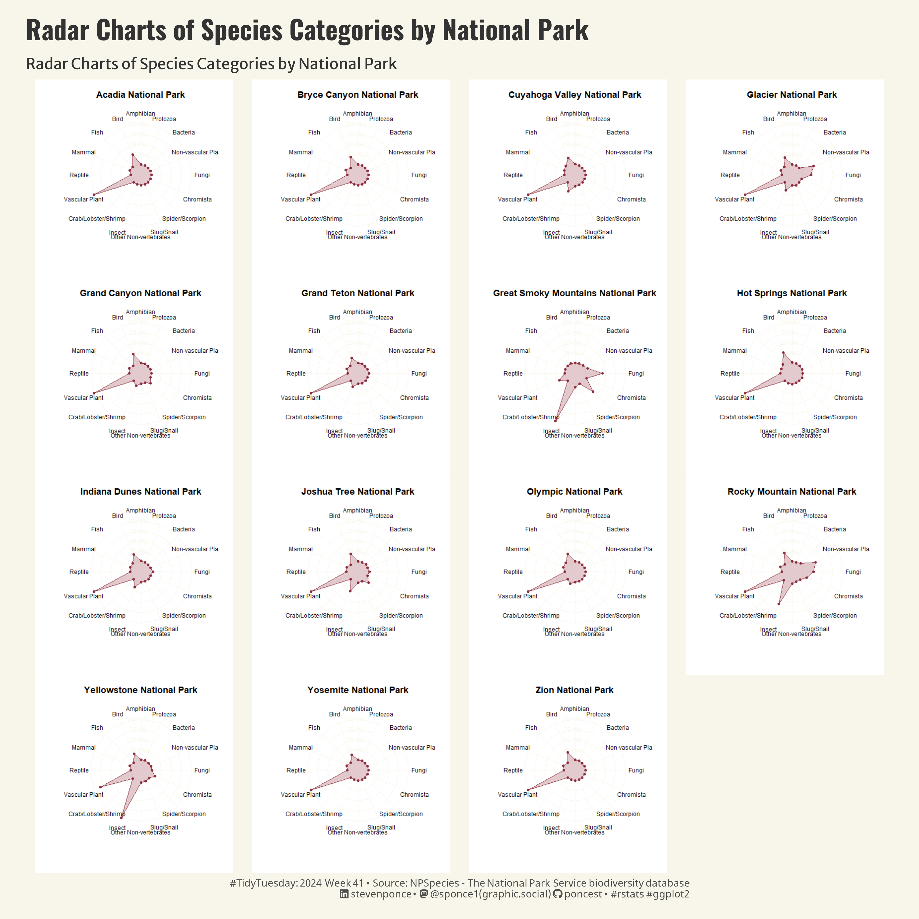
Radar Charts of Species Categories by National Park

Comparison of species distributions across U.S. national parks

Figure 1: The image displays 15 radar charts, with each chart representing different species categories in various U.S. national parks. Each chart is labeled with a park name and compares the counts of species such as mammals, reptiles, fungi, etc. These charts are used to visualize the biodiversity across the parks.”

Steps to Create this Graphic

1. Load Packages & Setup

```{r}
#| label: load

## 1. LOAD PACKAGES & SETUP ----
pacman::p_load(
    tidyverse,         # Easily Install and Load the 'Tidyverse'
    ggtext,            # Improved Text Rendering Support for 'ggplot2'
    showtext,          # Using Fonts More Easily in R Graphs
    janitor,           # Simple Tools for Examining and Cleaning Dirty Data
    skimr,             # Compact and Flexible Summaries of Data
    scales,            # Scale Functions for Visualization
    lubridate,         # Make Dealing with Dates a Little Easier
    glue,              # Interpreted String Literals
    fmsb,              # Functions for Medical Statistics Book with some Demographic Data
    purrr,             # Functional Programming Tools
    patchwork,         # The Composer of Plots
    grid,              # The Grid Graphics Package
    cowplot,           # Streamlined Plot Theme and Plot Annotations for 'ggplot2'
    png,               # Read and write PNG images
    here               # A Simpler Way to Find Your Files
)   

### |- figure size ---- 
camcorder::gg_record(
    dir    = here::here("temp_plots"),
    device = "png",
    width  =  10,
    height =  10,
    units  = "in",
    dpi    = 320
)

### |- resolution ----
showtext_opts(dpi = 320, regular.wt = 300, bold.wt = 800)
```

2. Read in the Data

```{r}
#| label: read

tt <-tidytuesdayR::tt_load(2024, week = 41) 

species_data <- tt$most_visited_nps_species_data |> clean_names() |> glimpse()

tidytuesdayR::readme(tt)
rm(tt)
```

3. Examing the Data

```{r}
#| label: examine

glimpse(species_data)
skim(species_data)
```

4. Tidy Data

```{r}
#| label: tidy

# Prepare data for radar plots
radar_data <- species_data |>
  count(park_name, category_name) |>
  pivot_wider(
    names_from = category_name,
    values_from = n,
    values_fill = 0
  )
```

5. Visualization Parameters

```{r}
#| label: params

### |- plot aesthetics ----
bkg_col      <- colorspace::lighten('#f7f5e9', 0.05)    
title_col    <- "gray20"           
subtitle_col <- "gray20"     
caption_col  <- "gray30"   
text_col     <- "gray20"    
col_palette  <- paletteer::paletteer_d("ButterflyColors::fountainea_ryphea")[c(1)] 

### |-  titles and caption ----
# icons
tt <- str_glue("#TidyTuesday: { 2024 } Week { 41 } &bull; Source: NPSpecies - The National Park Service biodiversity database<br>")
li <- str_glue("<span style='font-family:fa6-brands'>&#xf08c;</span>")
gh <- str_glue("<span style='font-family:fa6-brands'>&#xf09b;</span>")
mn <- str_glue("<span style='font-family:fa6-brands'>&#xf4f6;</span>")

# text
title_text    <- str_glue("Radar Charts of Species Categories by National Park")
subtitle_text <- str_glue("Comparison of species distributions across U.S. national parks")
caption_text  <- str_glue("{tt} {li} stevenponce &bull; {mn} @sponce1(graphic.social) {gh} poncest &bull; #rstats #ggplot2")

### |-  fonts ----
font_add("fa6-brands", "fonts/6.4.2/Font Awesome 6 Brands-Regular-400.otf")
font_add_google("Oswald", regular.wt = 400, family = "title")
font_add_google("Merriweather Sans", regular.wt = 400, family = "subtitle")
font_add_google("Merriweather Sans", regular.wt = 400, family = "text")
font_add_google("Noto Sans", regular.wt = 400, family = "caption")
showtext_auto(enable = TRUE)

### |-  plot theme ----
theme_set(theme_minimal(base_size = 14, base_family = "text"))                

theme_update(
    plot.title.position   = "plot",
    plot.caption.position = "plot",
    legend.position       = 'plot',
    plot.background       = element_rect(fill = bkg_col, color = bkg_col),
    panel.background      = element_rect(fill = bkg_col, color = bkg_col),
    plot.margin           = margin(t = 10, r = 20, b = 10, l = 20),
    
    axis.title.x          = element_text(margin = margin(10, 0, 0, 0), size = rel(1.1), 
                                         color = text_col, family = "text", face = "bold", hjust = 0.5),
    axis.title.y          = element_blank(),  
    axis.text.y           = element_blank(),
    axis.text.x           = element_text(color = text_col, family = "text", size = rel(0.9)),
    axis.ticks.x          = element_line(color = text_col),  
)

### |- plot function ----

# Function to create radar chart and save as PNG
create_and_save_radar_plot <- function(data, park_name) {
    
    # Define maximum and minimum values for the radar chart
    max_values <- rep(max(data), ncol(data))
    min_values <- rep(0, ncol(data))
    
    # Combine the max, min, and park data to create the radar chart data frame
    plot_data <- as.data.frame(rbind(max_values, min_values, data))
    colnames(plot_data) <- names(data)
    rownames(plot_data) <- c("Max", "Min", park_name)
    
     # Define the file path to save the radar chart
    temp_path <- here("2024/Week_41/")
    if (!dir.exists(temp_path)) {
      dir.create(temp_path, recursive = TRUE)
    }
    file_path <- file.path(temp_path, paste0("radar_plot_", gsub(" ", "_", park_name), ".png"))
    
    # Close any open devices
    while (!is.null(dev.list())) dev.off()
    
    # Create and save the radar chart as a PNG
    png(filename = file_path, width = 400, height = 400)
    fmsb::radarchart(plot_data,
                     axistype = 1,                             # Axis type configuration
                     title = park_name,                        # Title for the radar chart
                     pcol = col_palette,                       # Line color for the polygon
                     pfcol = scales::alpha(col_palette, 0.25), # Fill color for the polygon with transparency
                     plty = 1,                                 # Line type for the polygon
                     cglcol = bkg_col,                         # Color of the grid lines
                     cglty = 1,                                # Type of the grid lines
                     cglwd = 0.8,                              # Width of the grid lines
                     axislabcol = bkg_col,                     # Color of the axis labels
                     cex.axis = 1.2,                           # Increase axis text size
                     cex.main = 1.5                            # Increase title text size
    )
    dev.off()
    
    return(file_path)
}
```

6. Plot

```{r}
#| label: plot

### |-  individual plots ----
# Generate and save radar plots for each park
showtext_auto(enable = FALSE)
radar_plot_files <- radar_data |>
    split(radar_data$park_name) |>
    map_chr(~ {
        park_name <- .x$park_name[1]                      # Extract park name
        park_data <- .x |> select(-park_name)             # Remove park name column from data
        create_and_save_radar_plot(park_data, park_name)  # Create and save radar plot
    })


# Load each saved radar plot as a raster image and convert to ggplot
radar_plots <- map(radar_plot_files, ~ {
    img <- readPNG(.x)                                    # Read the saved PNG file
    ggdraw() + 
        draw_image(img)                                   # Convert the image to a ggplot object
    })


### |-  combined plots ----
showtext_auto(enable = TRUE)

combined_plot <- wrap_plots(radar_plots, ncol = 4) +
    plot_annotation(
        
        # Labs
        title = title_text,
        subtitle = title_text,
        caption = caption_text,
        
        # Theme
        theme = theme(
            plot.title = element_text(
                size = rel(1.7),
                family = "title",
                face = "bold",
                color = title_col,
                lineheight = 1.1,
                margin = margin(t = 5, b = 5)
            ),
            plot.subtitle = element_text(
                size = rel(1),
                family = "subtitle",
                color = subtitle_col,
                lineheight = 1.1,
                margin = margin(t = 5, b = 5)
            ),
            plot.caption = element_markdown(
                size = rel(0.65),
                family = "caption",
                color = caption_col,
                lineheight = 1.1,
                hjust = 0.5,
                halign = 1,
                margin = margin(t = 5, b = 5)
            )
        )
    )

combined_plot 
```

7. Save

```{r}
#| label: save

### |-  plot image ----  

library(ggplotify)
# Convert patchwork plot to grob 
# There was some issues between cowplot and ggsave
plot_grob <- as.grob(combined_plot)

# Save the plot again
# Activate showtext manually
showtext_begin()

# Save the plot as PNG
png(filename = here::here("data_visualizations/TidyTuesday/2024/tt_2024_41.png"),
    width = 10, height = 10, units = "in", res = 320)
grid.draw(plot_grob)
dev.off()

# Deactivate showtext
showtext_end()

### |-  plot thumbnail----  
magick::image_read(here::here("data_visualizations/TidyTuesday/2024/tt_2024_41.png")) |> 
  magick::image_resize(geometry = "400") |> 
  magick::image_write(here::here("data_visualizations/TidyTuesday/2024/thumbnails/tt_2024_41.png"))
```

8. Session Info

```{r, eval=TRUE}
info <- capture.output(sessioninfo::session_info())
# Remove lines that contain "[1]" and "[2]" (the file paths)
filtered_info <- grep("\\[1\\]|\\[2\\]", info, value = TRUE, invert = TRUE)
cat(filtered_info, sep = "\n")
```

─ Session info ───────────────────────────────────────────────────────────────
 setting  value
 version  R version 4.4.1 (2024-06-14 ucrt)
 os       Windows 11 x64 (build 22631)
 system   x86_64, mingw32
 ui       RTerm
 language (EN)
 collate  English_United States.utf8
 ctype    English_United States.utf8
 tz       America/New_York
 date     2025-05-22
 pandoc   3.4 @ C:/Program Files/RStudio/resources/app/bin/quarto/bin/tools/ (via rmarkdown)

─ Packages ───────────────────────────────────────────────────────────────────
 ! package     * version date (UTC) lib source
 P digest        0.6.37  2024-08-19 [?] RSPM (R 4.4.0)
 P evaluate      1.0.1   2024-10-10 [?] RSPM (R 4.4.0)
 P fastmap       1.2.0   2024-05-15 [?] RSPM (R 4.4.0)
 P htmltools     0.5.8.1 2024-04-04 [?] RSPM (R 4.4.0)
 P htmlwidgets   1.6.4   2023-12-06 [?] CRAN (R 4.4.0)
 P jsonlite      1.8.9   2024-09-20 [?] RSPM (R 4.4.0)
 P knitr         1.49    2024-11-08 [?] RSPM (R 4.4.0)
 P rmarkdown     2.29    2024-11-04 [?] RSPM (R 4.4.0)
 P rstudioapi    0.17.1  2024-10-22 [?] RSPM (R 4.4.0)
 P sessioninfo   1.2.2   2021-12-06 [?] RSPM (R 4.4.0)
 P xfun          0.49    2024-10-31 [?] RSPM (R 4.4.0)
 P yaml          2.3.10  2024-07-26 [?] RSPM (R 4.4.0)


 P ── Loaded and on-disk path mismatch.

──────────────────────────────────────────────────────────────────────────────