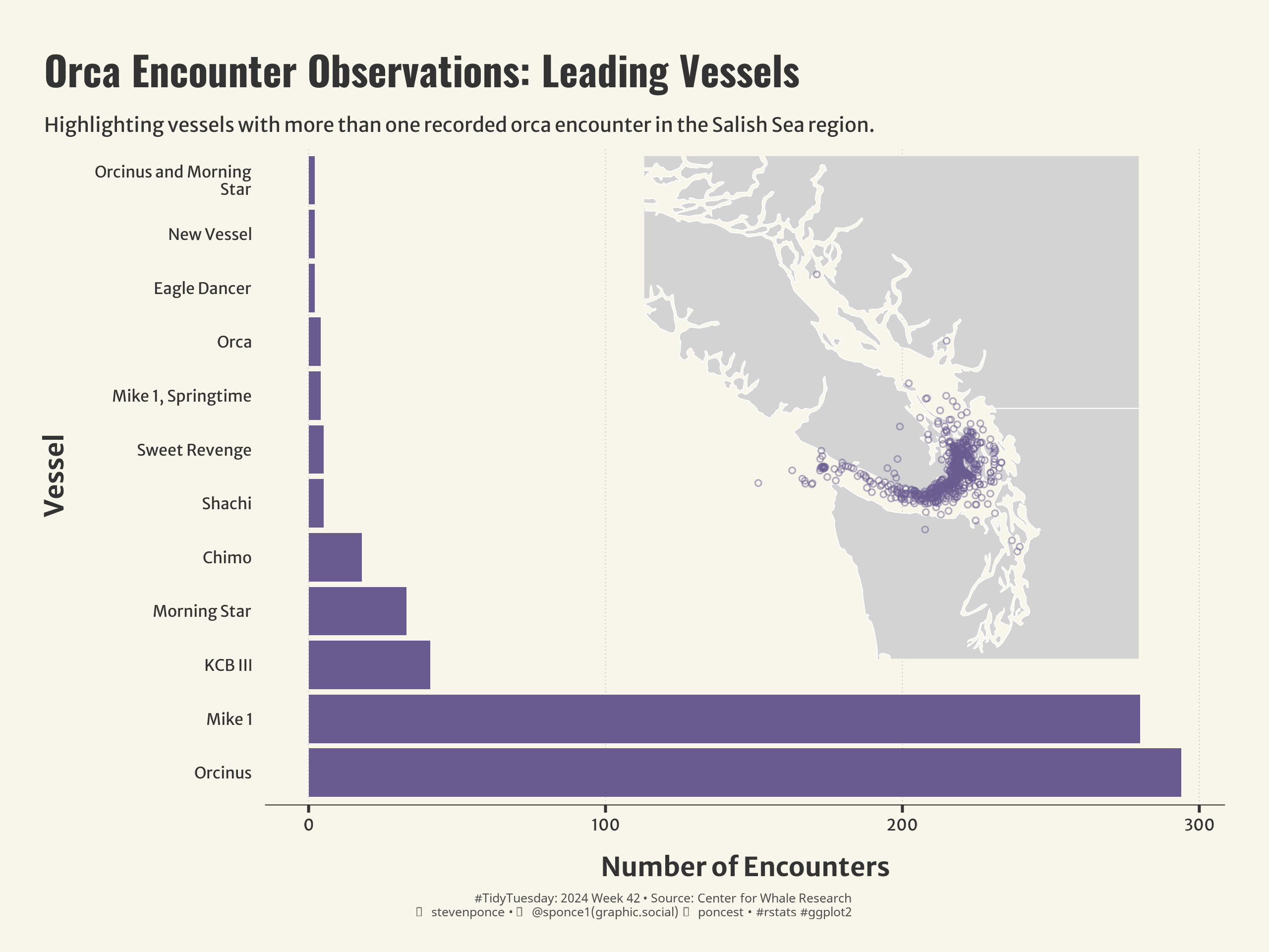
Orca Encounter Observations: Leading Vessels

Highlighting vessels with more than one recorded orca encounter in the Salish Sea region

Static

Figure 1: A bar chart displaying the number of orca encounters in the Salish Sea region, along with a map showing the locations of the encounters. Orcinus and Mike 1 are the vessels with the highest number of encounters, each exceeding 200.

NOTE: We used runtime: shiny to make the interactive features of our visualizations work smoothly, especially the interactive orca map. This let us add dynamic, user-driven exploration that wasn’t possible with the usual Quarto options (I needed help figuring it out!).

While it means the final result looks more like markdown and less like a sleek Quarto document, it was the best way to ensure the interactivity worked well.

Steps to Create this Graphic

1. Load Packages & Setup

```{r}
#| label: load
#| warning: false

## 1. LOAD PACKAGES & SETUP ----
pacman::p_load(
    tidyverse,         # Easily Install and Load the 'Tidyverse'
    ggtext,            # Improved Text Rendering Support for 'ggplot2'
    showtext,          # Using Fonts More Easily in R Graphs
    janitor,           # Simple Tools for Examining and Cleaning Dirty Data
    skimr,             # Compact and Flexible Summaries of Data
    scales,            # Scale Functions for Visualization
    lubridate,         # Make Dealing with Dates a Little Easier
    glue,              # Interpreted String Literals
    patchwork,         # The Composer of Plots
    here,              # A Simpler Way to Find Your Files
    sf,                # Simple Features for R
    ggiraph,           # Make 'ggplot2' Graphics Interactive
    htmltools,         # Tools for HTML
    rnaturalearth,     # World Map Data from Natural Earth 
    rnaturalearthhires # High Resolution World Vector Map Data from Natural Earth used inrnaturalearth
)  

# Note: disabled { camcorder }. Issues with plot rendering (ggiraph)

# ### |- figure size ---- 
# camcorder::gg_record(
#     dir    = here::here("temp_plots"),
#     device = "png",
#     width  =  10,
#     height =  10,
#     units  = "in",
#     dpi    = 320
# )

### |- resolution ----
showtext_opts(dpi = 320, regular.wt = 300, bold.wt = 800)
```

2. Read in the Data

```{r}
#| label: read
#| include: true
#| eval: true
#| warning: false

tt <-tidytuesdayR::tt_load(2024, week = 42) 

orcas_data <- tt$orcas |> clean_names() 

tidytuesdayR::readme(tt)
rm(tt)
```

3. Examine the Data

```{r}
#| label: examine
#| include: true
#| eval: true
#| results: 'hide'
#| warning: false

glimpse(orcas_data)
```

4. Tidy Data

```{r}
#| label: tidy
#| warning: false

### |- tidy data ----
orcas_data_clean <- orcas_data |>
    filter(!is.na(vessel)) |>
    # Standardize 'ids_encountered' to be comma-separated
    mutate(
        ids_encountered = str_replace_all(ids_encountered, "and", ","),
        ids_encountered = str_replace_all(ids_encountered, ",[[:space:]]*", ", "),
        ids_encountered = str_trim(ids_encountered)
    ) |>  
    # Extract numeric duration from the 'duration' column and convert to minutes
    mutate(
        duration_minutes = str_extract(duration, "[[:digit:]]+") |> as.numeric() / 60,
        duration_minutes = ifelse(duration_minutes < 0, NA, duration_minutes)
    ) |>
    # Convert 'date' to proper Date class and create month column
    mutate(
        date = as.Date(date),
        month = month(date, label = TRUE, abbr = FALSE)
    ) |>
    # Handle missing values
    filter(!is.na(encounter_number), !is.na(begin_latitude), !is.na(begin_longitude))


# ### |- data for bar plot ----

# Number of Encounters per Vessel
bar_plot_data <- orcas_data_clean |>
    filter(!is.na(vessel)) |>
    count(vessel, sort = TRUE) |>
    filter(n > 1) |>
    mutate(
        vessel = str_wrap(vessel, width = 20),
        vessel = fct_reorder(vessel, -n)
    )
```

5. Visualization Parameters

```{r}
#| label: params
#| include: true
#| warning: false

### |- plot aesthetics ----
bkg_col      <- colorspace::lighten('#f7f5e9', 0.05)    
title_col    <- "gray20"           
subtitle_col <- "gray20"     
caption_col  <- "gray30"   
text_col     <- "gray20"    
col_palette  <- paletteer::paletteer_d("lisa::OdilonRedon")[c(1,2)] 
# show_col(col_palette)

### |-  titles and caption ----
# icons
tt <- str_glue("#TidyTuesday: { 2024 } Week { 42 } &bull; Source: Center for Whale Research<br>")
li <- str_glue("<span style='font-family:fa6-brands'>&#xf08c;</span>")
gh <- str_glue("<span style='font-family:fa6-brands'>&#xf09b;</span>")
mn <- str_glue("<span style='font-family:fa6-brands'>&#xf4f6;</span>")

# text
title_text    <- str_glue("Orca Encounter Observations: Leading Vessels")
subtitle_text <- str_glue("Highlighting vessels with more than one recorded orca encounter in the Salish Sea region.")
caption_text  <- str_glue("{tt} {li} stevenponce &bull; {mn} @sponce1(graphic.social) {gh} poncest &bull; #rstats #ggplot2")

### |-  fonts ----
# font_add("fa6-brands", "personal-website/fonts/6.4.2/Font Awesome 6 Brands-Regular-400.otf")
font_add_google("Oswald", regular.wt = 400, family = "title")
font_add_google("Merriweather Sans", regular.wt = 400, family = "subtitle")
font_add_google("Merriweather Sans", regular.wt = 400, family = "text")
font_add_google("Noto Sans", regular.wt = 400, family = "caption")
showtext_auto(enable = TRUE)

### |-  plot theme ----
theme_set(theme_minimal(base_size = 14, base_family = "text"))                

theme_update(
    plot.title.position   = "plot",
    plot.caption.position = "plot",
    legend.position       = 'plot',
    
    plot.background       = element_rect(fill = bkg_col, color = bkg_col),
    panel.background      = element_rect(fill = bkg_col, color = bkg_col),
    plot.margin           = margin(t = 10, r = 10, b = 5, l = 10),
    
    panel.grid.minor      = element_blank(),
    panel.grid.major.y    = element_blank(),
    panel.grid.major.x    = element_line(linetype = "dotted", linewidth = 0.2, color = 'gray'),
    
    axis.title.x          = element_text(margin = margin(10, 0, 0, 0), size = rel(0.85), 
                                         color = text_col, family = "text", face = "bold", hjust = 0.5),
    axis.title.y          = element_text(margin = margin(0, 10, 0, 0), size = rel(0.85), 
                                         color = text_col, family = "text", face = "bold", hjust = 0.5),
    
    axis.text.y           = element_text(color = text_col, family = "text", size = rel(0.65)),
    axis.text.x           = element_text(color = text_col, family = "text", size = rel(0.65)),
    
    axis.ticks.x          = element_line(color = text_col),  
    axis.line.x           = element_line(color = "#252525", linewidth = .2)
)
```

6. Plot (Interactive)

```{r}
#| label: plot
#| warning: false

### |- world map for background ----
world <- st_as_sf(rnaturalearth::ne_countries(scale = 'large', returnclass = 'sf'))

### |- Base map ----

# Focus on the Salish Sea region
map <- ggplot() +
    
    # Geoms
    geom_sf(data = world, fill = "lightgrey", color = "white") +
    geom_sf_interactive(
        data = st_as_sf(orcas_data_clean, coords = c("begin_longitude", "begin_latitude"), crs = 4326),
        aes(tooltip = paste("Date:", date, "<br>Location:", location), data_id = vessel), 
        color = col_palette[1],
        alpha = 0.5,
        shape = 1,
        size = 1
    ) +
    
    # Scales
    coord_sf(xlim = c(-127, -121), ylim = c(47, 51), expand = FALSE) +          # Focus on the Salish Sea region
    
    # Labs 
    labs(
        title = "",
        x = "Longitude",
        y = "Latitude"
    ) +
    
    # Theme
    ggthemes::theme_map() 


### |- Bar plot plot ----

# Number of Encounters per Vessel
bar <- ggplot(bar_plot_data, aes(x = vessel, -n, y = n)) +
    
    # Geom
    geom_bar_interactive(
        aes(
            tooltip = paste("Vessel:", vessel, "<br>Encounters:", n), 
            data_id = vessel), 
        stat = "identity", 
        fill = col_palette[1]
    ) +
    
    # Scale
    scale_x_discrete() +
    scale_y_continuous() +    
    coord_flip() +
    
    # Labs
    labs(
        x = "Vessel",
        y = "Number of Encounters",
        title = title_text,
        subtitle = subtitle_text,
        caption = caption_text
    )  +
    
    # Theme
    theme(
        plot.title = element_text(
            size = rel(1.3),
            family = "title",
            face = "bold",
            color = title_col,
            lineheight = 1.1,
            margin = margin(t = 5, b = 5)
        ),
        plot.subtitle = element_text(
            size = rel(0.65),
            family = "subtitle",
            color = subtitle_col,
            lineheight = 1.1,
            margin = margin(t = 5, b = 5)
        ),
        plot.caption = element_markdown(    
            size = rel(0.40),
            family = "caption", 
            color = caption_col,
            lineheight = 1.1,
            hjust = 0.5,
            halign = 1,
            margin = margin(t = 5, b = 5)
        )
    )

### |- inset element ----

# Insert the map into the upper right corner of the bar plot 
combined_plot <- bar + 
    inset_element(map, left = 0, bottom = 0.2, right = 1.3, top = 1.05)
```

```{r}
#| label: interactive
#| eval: true
#| include: true
#| fig.width: 8
#| fig.height: 6
#| warning: false

### |-  interactive plots ----

# Create the interactive plot with ggiraph
interactive_plot <- girafe(
  ggobj = combined_plot,
  bg = bkg_col,
  options = list(
    opts_tooltip(
      opacity = 0.8, use_fill = TRUE,
      use_stroke = FALSE,
      css = "padding:5pt;font-family: 'Open Sans', sans-serif;font-size:1.2rem;color:white"),
    opts_selection(type = "single", css = "fill:yellow;stroke:black;stroke-width:2px;"),
    opts_sizing(rescale = TRUE),
    opts_toolbar(saveaspng = TRUE),
    opts_hover_inv(css = "opacity:0.4"),
    opts_hover(
      css = girafe_css(
        css = glue("fill:{col_palette[2]};"),
        text = "stroke:none;fill:white;fill-opacity:1;")
    )
  )
)

# Use tagList to render it properly in Quarto
htmltools::tagList(interactive_plot)
```

Note: This chart was inspired by Yan Holtz (@R_Graph_Gallery) “Combine charts in ggiraph” post that can be found HERE

7. Save

```{r}
#| label: save
#| warning: false

### |-  plot image ----  

# Save the plot as PNG
ggsave(
  filename = here::here("data_visualizations/TidyTuesday/2024/tt_2024_42.png"), 
  plot = combined_plot,
  width = 8, height = 6, units = "in", dpi = 320
)

### |-  plot thumbnail----  
magick::image_read(here::here("data_visualizations/TidyTuesday/2024/tt_2024_42.png")) |> 
  magick::image_resize(geometry = "400") |> 
  magick::image_write(here::here("data_visualizations/TidyTuesday/2024/thumbnails/tt_2024_42.png"))
```

8. Session Info

TipExpand for Session Info

R version 4.4.1 (2024-06-14 ucrt)
Platform: x86_64-w64-mingw32/x64
Running under: Windows 11 x64 (build 22631)

Matrix products: default


locale:
[1] LC_COLLATE=English_United States.utf8 
[2] LC_CTYPE=English_United States.utf8   
[3] LC_MONETARY=English_United States.utf8
[4] LC_NUMERIC=C                          
[5] LC_TIME=English_United States.utf8    

time zone: America/New_York
tzcode source: internal

attached base packages:
[1] stats     graphics  grDevices datasets  utils     methods   base     

other attached packages:
 [1] rnaturalearthhires_1.0.0.9000 rnaturalearth_1.0.1          
 [3] htmltools_0.5.8.1             ggiraph_0.8.10               
 [5] sf_1.0-19                     here_1.0.1                   
 [7] patchwork_1.3.0               glue_1.8.0                   
 [9] scales_1.3.0                  skimr_2.1.5                  
[11] janitor_2.2.0                 showtext_0.9-7               
[13] showtextdb_3.0                sysfonts_0.8.9               
[15] ggtext_0.1.2                  lubridate_1.9.3              
[17] forcats_1.0.0                 stringr_1.5.1                
[19] dplyr_1.1.4                   purrr_1.0.2                  
[21] readr_2.1.5                   tidyr_1.3.1                  
[23] tibble_3.2.1                  ggplot2_3.5.1                
[25] tidyverse_2.0.0              

loaded via a namespace (and not attached):
 [1] tidyselect_1.2.1   farver_2.1.2       fastmap_1.2.0      gh_1.4.1          
 [5] pacman_0.5.1       digest_0.6.37      timechange_0.3.0   lifecycle_1.0.4   
 [9] terra_1.7-83       magrittr_2.0.3     compiler_4.4.0     rlang_1.1.6       
[13] tools_4.4.0        utf8_1.2.4         yaml_2.3.10        knitr_1.49        
[17] labeling_0.4.3     htmlwidgets_1.6.4  bit_4.5.0          classInt_0.4-10   
[21] curl_6.0.0         xml2_1.3.6         repr_1.1.7         KernSmooth_2.23-22
[25] tidytuesdayR_1.1.2 withr_3.0.2        grid_4.4.0         fansi_1.0.6       
[29] e1071_1.7-16       colorspace_2.1-1   paletteer_1.6.0    gitcreds_0.1.2    
[33] cli_3.6.4          rmarkdown_2.29     crayon_1.5.3       ragg_1.3.3        
[37] generics_0.1.3     rstudioapi_0.17.1  httr_1.4.7         tzdb_0.5.0        
[41] commonmark_1.9.2   DBI_1.2.3          proxy_0.4-27       ggthemes_5.1.0    
[45] parallel_4.4.0     base64enc_0.1-3    vctrs_0.6.5        jsonlite_1.8.9    
[49] hms_1.1.3          bit64_4.5.2        magick_2.8.5       systemfonts_1.1.0 
[53] units_0.8-5        rematch2_2.1.2     codetools_0.2-20   stringi_1.8.4     
[57] gtable_0.3.6       prismatic_1.1.2    munsell_0.5.1      pillar_1.9.0      
[61] rappdirs_0.3.3     R6_2.5.1           httr2_1.0.6        textshaping_0.4.0 
[65] rprojroot_2.0.4    vroom_1.6.5        evaluate_1.0.1     markdown_1.13     
[69] gridtext_0.1.5     snakecase_0.11.1   renv_1.0.3         class_7.3-22      
[73] Rcpp_1.0.13-1      uuid_1.2-1         xfun_0.49          pkgconfig_2.0.3   

9. GitHub Repository

TipExpand for GitHub Repo

Access the GitHub repository here