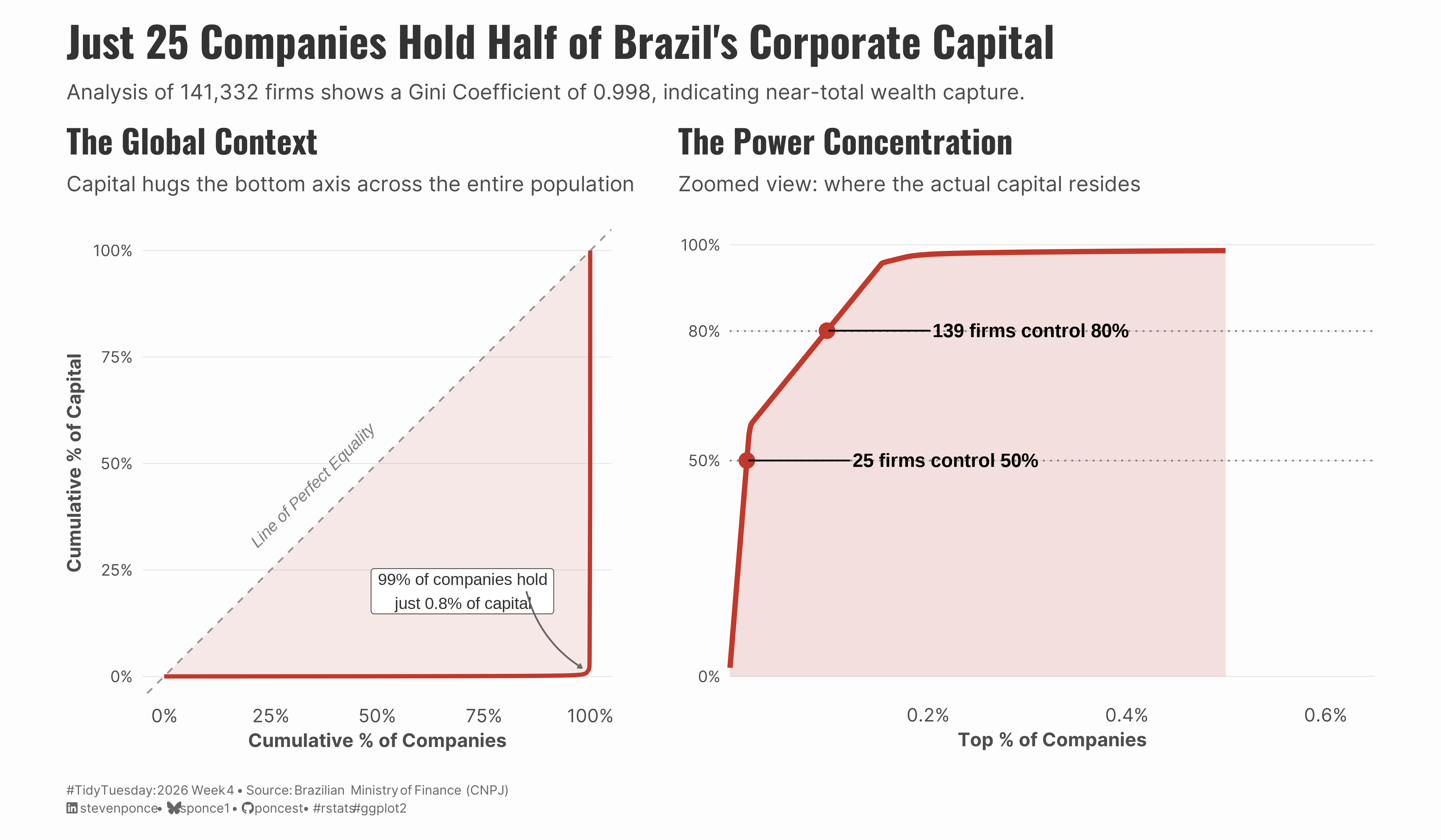
Just 25 Companies Hold Half of Brazil’s Corporate Capital

Analysis of 141,332 firms shows a Gini Coefficient of 0.998, indicating near-total wealth capture.

This visualization explores corporate capital concentration in Brazil using Lorenz curve analysis of 141,332 companies from the CNPJ open registry. A dual-panel approach reveals extreme inequality: the traditional Lorenz curve shows capital hugging the bottom axis, while a zoomed view of the top 0.6% exposes that just 25 companies control half of all corporate capital.

Figure 1: Dual-panel Lorenz curve visualization showing extreme corporate capital concentration in Brazil. The left panel displays a traditional Lorenz curve in which the red line hugs the bottom axis, indicating that 99% of companies hold just 0.8% of total capital, with a diagonal dashed line representing perfect equality. The right panel zooms in on the top 0.6% of companies, revealing that just 25 firms control 50% of all capital, and 139 firms control 80%. The Gini coefficient of 0.998 indicates near-total wealth capture among 141,332 registered Brazilian companies.

Steps to Create this Graphic

1. Load Packages & Setup

```{r}
#| label: load
#| warning: false
#| message: false
#| results: "hide"

## 1. LOAD PACKAGES & SETUP ----
suppressPackageStartupMessages({
if (!require("pacman")) install.packages("pacman")
pacman::p_load(
    tidyverse, ggtext, showtext, janitor, 
    scales, glue, patchwork, ineq, ggrepel
)
})

### |- figure size ----
camcorder::gg_record(
  dir    = here::here("temp_plots"),
  device = "png",
  width  = 12,
  height = 7,
  units  = "in",
  dpi    = 320
)

# Source utility functions
suppressMessages(source(here::here("R/utils/fonts.R")))
source(here::here("R/utils/social_icons.R"))
source(here::here("R/utils/image_utils.R"))
source(here::here("R/themes/base_theme.R"))
```

2. Read in the Data

```{r}
#| label: read
#| include: true
#| eval: true
#| warning: false

tt <- tidytuesdayR::tt_load(2026, week = 04)
companies <- tt$companies |> clean_names()
rm(tt)
```

3. Examine the Data

```{r}
#| label: examine
#| include: true
#| eval: true
#| results: 'hide'
#| warning: false

glimpse(companies)
```

4. Tidy Data

```{r}
#| label: tidy
#| warning: false

companies_clean <- companies |>
  mutate(capital_stock = replace_na(capital_stock, 0))

n_companies <- nrow(companies_clean)
gini_val <- Gini(companies_clean$capital_stock)

# Lorenz Data (Bottom-Up)
lorenz_bottom <- companies_clean |>
  arrange(capital_stock) |>
  mutate(
    cum_companies = row_number() / n(),
    cum_capital = cumsum(capital_stock) / sum(capital_stock)
  )

# Pareto Data (Top-Down Zoom)
lorenz_top <- companies_clean |>
  arrange(desc(capital_stock)) |>
  mutate(
    top_pct_companies = row_number() / n(),
    cum_capital = cumsum(capital_stock) / sum(capital_stock)
  )

# Thresholds
p99 <- lorenz_bottom |> filter(cum_companies >= 0.99) |> slice_head(n = 1)
hold_50 <- lorenz_top |> filter(cum_capital >= 0.50) |> slice_head(n = 1)
hold_80 <- lorenz_top |> filter(cum_capital >= 0.80) |> slice_head(n = 1)
n_25 <- round(hold_50$top_pct_companies * n_companies)
```

5. Visualization Parameters

```{r}
#| label: params
#| include: true
#| warning: false

### |-  plot aesthetics ----
colors <- get_theme_colors(
  palette = list(
      col_curve <- "#c0392b"   
  )
)

### |- titles and caption ----
title_text = str_glue("Just {n_25} Companies Hold Half of Brazil's Corporate Capital")

subtitle_text = str_glue(
    "Analysis of {comma(n_companies)} firms shows a Gini Coefficient of {round(gini_val, 3)}, indicating near-total wealth capture."
    )

caption_text <- create_social_caption(
    tt_year = 2026,
    tt_week = 04,
    source_text = "Brazilian Ministry of Finance (CNPJ)"
)

### |-  fonts ----
setup_fonts()
fonts <- get_font_families()

### |-  plot theme ----
# Start with base theme
base_theme <- create_base_theme(colors)

# Add weekly-specific theme elements
weekly_theme <- extend_weekly_theme(
  base_theme,
  theme(
    # Text styling
    plot.title = element_text(
      face = "bold", family = fonts$title, size = rel(1.4),
      color = colors$title, margin = margin(b = 10), hjust = 0
    ),
    plot.subtitle = element_text(
      face = "italic", family = fonts$subtitle, lineheight = 1.2,
      color = colors$subtitle, size = rel(0.9), margin = margin(b = 20), hjust = 0
    ),

    # Grid
    panel.grid.minor = element_blank(),
    panel.grid.major.x = element_blank(),
    panel.grid.major = element_line(color = "gray90", linewidth = 0.25),

    # Axes
    axis.title = element_text(size = rel(0.8), color = "gray30"),
    axis.text = element_text(color = "gray30"),
    axis.text.y = element_text(size = rel(0.85)),
    axis.ticks = element_blank(),

    # Facets
    strip.background = element_rect(fill = "gray95", color = NA),
    strip.text = element_text(
      face = "bold",
      color = "gray20",
      size = rel(0.9),
      margin = margin(t = 6, b = 4)
    ),
    panel.spacing = unit(1.5, "lines"),

    # Legend elements
    legend.position = "plot",
    legend.title = element_text(
      family = fonts$subtitle,
      color = colors$text, size = rel(0.8), face = "bold"
    ),
    legend.text = element_text(
      family = fonts$tsubtitle,
      color = colors$text, size = rel(0.7)
    ),
    legend.margin = margin(t = 15),

    # Plot margin
    plot.margin = margin(10, 20, 10, 20),
    
  )
)

# Set theme
theme_set(weekly_theme)
```

6. Plot

```{r}
#| label: plot
#| warning: false

### |- LEFT PANEL: THE MACRO PROBLEM ----
panel_left <- lorenz_bottom |>
  # Geoms
  ggplot(aes(x = cum_companies, y = cum_capital)) +
  geom_abline(slope = 1, intercept = 0, linetype = "dashed", color = "gray60") +
  geom_ribbon(aes(ymin = cum_capital, ymax = cum_companies), alpha = 0.1, fill = col_curve) +
  geom_line(color = col_curve, linewidth = 1.2) +
  # Annotations
  annotate("text",
    x = 0.35, y = 0.45, label = "Line of Perfect Equality",
    angle = 45, size = 3.5, color = "gray50", fontface = "italic"
  ) +
  annotate("label",
    x = 0.70, y = 0.20,
    label = glue("99% of companies hold\njust {percent(p99$cum_capital, 0.1)} of capital"),
    fill = "white", color = "gray20", size = 3.5, label.size = 0.2
  ) +
  annotate("curve",
    x = 0.85, y = 0.20, xend = 0.98, yend = 0.02,
    curvature = 0.2, color = "gray40", arrow = arrow(length = unit(0.1, "cm"))
  ) +
  # Scales
  scale_x_continuous(labels = percent_format()) +
  scale_y_continuous(labels = percent_format()) +
  coord_fixed() +
  # Labs
  labs(
    title = "The Global Context",
    subtitle = "Capital hugs the bottom axis across the entire population",
    x = "Cumulative % of Companies",
    y = "Cumulative % of Capital"
  )

### |- RIGHT PANEL: THE POWER CONCENTRATION----
panel_right <- lorenz_top |>
  filter(top_pct_companies <= 0.005) |>
  # Geoms
  ggplot(aes(x = top_pct_companies, y = cum_capital)) +
  geom_area(fill = col_curve, alpha = 0.15) +
  geom_hline(yintercept = c(0.5, 0.8), linetype = "dotted", color = "gray50") +
  geom_line(color = col_curve, linewidth = 1.5) +
  geom_point(data = bind_rows(hold_50, hold_80), size = 4, color = col_curve) +
  geom_text_repel(
    data = bind_rows(hold_50, hold_80),
    aes(label = glue("{comma(round(top_pct_companies * n_companies))} firms control {percent(cum_capital)}")),
    nudge_x = 0.001, direction = "y", hjust = 0, size = 4, fontface = "bold"
  ) +
  # Scales
  scale_x_continuous(labels = percent_format(accuracy = 0.1), expand = expansion(mult = c(0, 0.3))) +
  scale_y_continuous(labels = percent_format(), breaks = c(0, 0.5, 0.8, 1)) +
  coord_cartesian(clip = "off") +
  # Labs
  labs(
    title = "The Power Concentration",
    subtitle = "Zoomed view: where the actual capital resides",
    x = "Top % of Companies",
    y = NULL
  )

### |- COMBINE ----
combined_plot <-(panel_left + panel_right) +
    plot_annotation(
        title = title_text,
        subtitle = subtitle_text,
        caption = caption_text,
        theme = theme(
    plot.title = element_text(
      size = rel(1.8),
      family = fonts$title,
      face = "bold",
      color = colors$title,
      lineheight = 1.15,
      margin = margin(t = 5, b = 5)
    ),
    plot.subtitle = element_text(
      size = rel(0.9),
      family = fonts$subtitle,
      color = colors$subtitle,
      lineheight = 1.5,
      margin = margin(t = 5, b = 5)
    ),
    plot.caption = element_markdown(
      size = rel(0.55),
      family = fonts$subtitle,
      color = colors$caption,
      hjust = 0,
      lineheight = 1.4,
      margin = margin(t = 10, b = 5)
    ),
  )
)
```

7. Save

```{r}
#| label: save
#| warning: false

### |-  plot image ----  
save_plot_patchwork(
  plot = combined_plot, 
  type = "tidytuesday", 
  year = 2026, 
  week = 04, 
  width  = 12,
  height = 7,
  )
```

8. Session Info

TipExpand for Session Info

R version 4.4.1 (2024-06-14 ucrt)
Platform: x86_64-w64-mingw32/x64
Running under: Windows 11 x64 (build 26100)

Matrix products: default


locale:
[1] LC_COLLATE=English_United States.utf8 
[2] LC_CTYPE=English_United States.utf8   
[3] LC_MONETARY=English_United States.utf8
[4] LC_NUMERIC=C                          
[5] LC_TIME=English_United States.utf8    

time zone: America/New_York
tzcode source: internal

attached base packages:
[1] stats     graphics  grDevices datasets  utils     methods   base     

other attached packages:
 [1] here_1.0.1      ggrepel_0.9.6   ineq_0.2-13     patchwork_1.3.0
 [5] glue_1.8.0      scales_1.3.0    janitor_2.2.0   showtext_0.9-7 
 [9] showtextdb_3.0  sysfonts_0.8.9  ggtext_0.1.2    lubridate_1.9.3
[13] forcats_1.0.0   stringr_1.5.1   dplyr_1.1.4     purrr_1.0.2    
[17] readr_2.1.5     tidyr_1.3.1     tibble_3.2.1    ggplot2_3.5.1  
[21] tidyverse_2.0.0 pacman_0.5.1   

loaded via a namespace (and not attached):
 [1] gtable_0.3.6       httr2_1.0.6        xfun_0.49          htmlwidgets_1.6.4 
 [5] gh_1.4.1           tzdb_0.5.0         yulab.utils_0.1.8  vctrs_0.6.5       
 [9] tools_4.4.0        generics_0.1.3     parallel_4.4.0     curl_6.0.0        
[13] gifski_1.32.0-1    fansi_1.0.6        pkgconfig_2.0.3    ggplotify_0.1.2   
[17] lifecycle_1.0.4    compiler_4.4.0     farver_2.1.2       munsell_0.5.1     
[21] codetools_0.2-20   snakecase_0.11.1   htmltools_0.5.8.1  yaml_2.3.10       
[25] crayon_1.5.3       pillar_1.9.0       camcorder_0.1.0    magick_2.8.5      
[29] commonmark_1.9.2   tidyselect_1.2.1   digest_0.6.37      stringi_1.8.4     
[33] labeling_0.4.3     rsvg_2.6.1         rprojroot_2.0.4    fastmap_1.2.0     
[37] grid_4.4.0         colorspace_2.1-1   cli_3.6.4          magrittr_2.0.3    
[41] utf8_1.2.4         withr_3.0.2        rappdirs_0.3.3     bit64_4.5.2       
[45] timechange_0.3.0   rmarkdown_2.29     tidytuesdayR_1.1.2 gitcreds_0.1.2    
[49] bit_4.5.0          hms_1.1.3          evaluate_1.0.1     knitr_1.49        
[53] markdown_1.13      gridGraphics_0.5-1 rlang_1.1.6        gridtext_0.1.5    
[57] Rcpp_1.0.13-1      xml2_1.3.6         renv_1.0.3         vroom_1.6.5       
[61] svglite_2.1.3      rstudioapi_0.17.1  jsonlite_1.8.9     R6_2.5.1          
[65] fs_1.6.5           systemfonts_1.1.0 

9. GitHub Repository

TipExpand for GitHub Repo

The complete code for this analysis is available in tt_2026_04.qmd.

For the full repository, click here.

10. References

TipExpand for References

1. Data Source:
   • TidyTuesday 2026 Week 04: Brazilian Companies
   • Brazilian Ministry of Finance: CNPJ Open Data
   • Data Dictionary: CNPJ Metadata (PDF)
2. Methodology:
   • Lorenz Curve: Wikipedia
   • Gini Coefficient: Wikipedia
   • R Package ineq: CRAN Documentation

11. Custom Functions Documentation

Note📦 Custom Helper Functions

This analysis uses custom functions from my personal module library for efficiency and consistency across projects.

Functions Used:

• fonts.R: setup_fonts(), get_font_families() - Font management with showtext
• social_icons.R: create_social_caption() - Generates formatted social media captions
• image_utils.R: save_plot() - Consistent plot saving with naming conventions
• base_theme.R: create_base_theme(), extend_weekly_theme(), get_theme_colors() - Custom ggplot2 themes

Why custom functions?
These utilities standardize theming, fonts, and output across all my data visualizations. The core analysis (data tidying and visualization logic) uses only standard tidyverse packages.

Source Code:
View all custom functions → GitHub: R/utils