From Seed to Table: How Long Until Harvest?

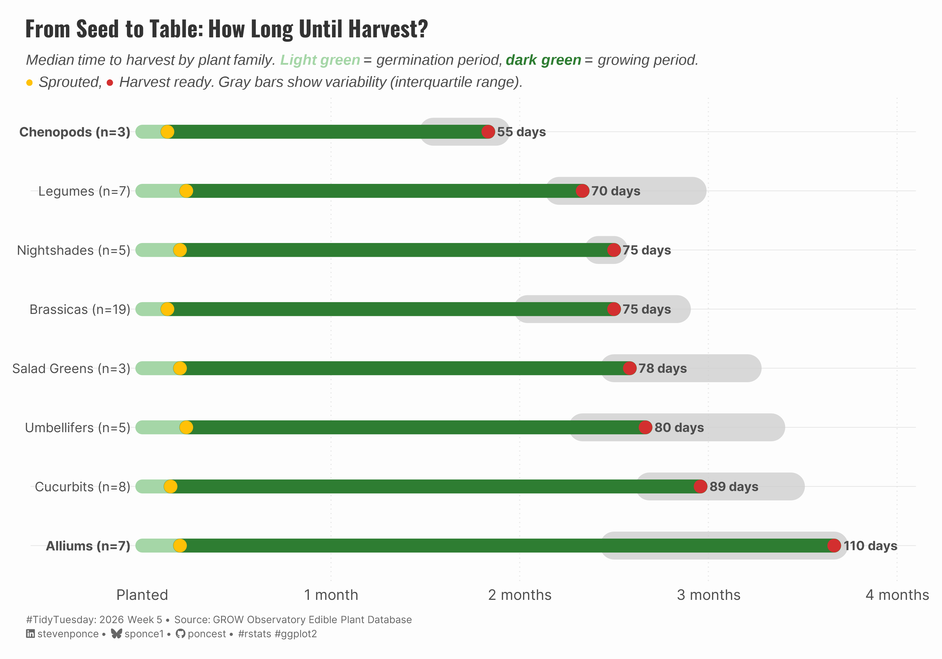
Median time to harvest by plant family. Light green = germination period, dark green = growing period. ● Sprouted, ● Harvest ready. Gray bars show variability (interquartile range).

A horizontal bar chart visualizing median growing timelines for nine edible plant families, from planting to harvest. Chenopods are the fastest at 55 days while Alliums take the longest at 110 days. Built with R and ggplot2 using data from the GROW Observatory Edible Plant Database.

Figure 1: Bar chart showing harvest timelines for 9 plant families. Chenopods are fastest (55 days), Alliums slowest (110 days). Light green = germination, dark green = growing period. Gray bars show variability. Source: GROW Observatory.

Steps to Create this Graphic

1. Load Packages & Setup

```{r}
#| label: load
#| warning: false
#| message: false
#| results: "hide"

## 1. LOAD PACKAGES & SETUP ----
suppressPackageStartupMessages({
if (!require("pacman")) install.packages("pacman")
pacman::p_load(
    tidyverse, ggtext, showtext, janitor, 
    scales, glue, patchwork, ineq, ggrepel
)
})

### |- figure size ----
camcorder::gg_record(
  dir    = here::here("temp_plots"),
  device = "png",
  width  = 10,
  height = 7,
  units  = "in",
  dpi    = 320
)

# Source utility functions
suppressMessages(source(here::here("R/utils/fonts.R")))
source(here::here("R/utils/social_icons.R"))
source(here::here("R/utils/image_utils.R"))
source(here::here("R/themes/base_theme.R"))
```

2. Read in the Data

```{r}
#| label: read
#| include: true
#| eval: true
#| warning: false

tt <- tidytuesdayR::tt_load(2026, week = 05)
edible_plants <- tt$edible_plants |> clean_names()
rm(tt)
```

3. Examine the Data

```{r}
#| label: examine
#| include: true
#| eval: true
#| results: 'hide'
#| warning: false

glimpse(edible_plants)
```

4. Tidy Data

```{r}
#| label: tidy
#| warning: false

# Helper: parse numeric ranges like "55-75", "55 – 75"...
parse_range <- function(x, return = c("midpoint", "lower", "upper")) {
  return <- match.arg(return)

  map_dbl(x, function(val) {
    if (is.na(val) || val == "") {
      return(NA_real_)
    }

    val <- str_trim(val)
    val <- str_to_lower(val)

    # Standardize separators
    val <- str_replace_all(val, c("–" = "-", "—" = "-", " to " = "-", "–" = "-"))
    val <- str_replace_all(val, "[^0-9\\.-]+", "") # keep digits, dot, dash

    # Handle "~75" style after stripping non-numeric (becomes "75")
    if (str_detect(val, "^\\d+\\.?\\d*\\+$")) {
      num <- as.numeric(str_remove(val, "\\+$"))
      return(case_when(
        return == "midpoint" ~ num,
        return == "lower" ~ num,
        return == "upper" ~ NA_real_
      ))
    }

    if (str_detect(val, "^\\d+\\.?\\d*-$")) {
      num <- as.numeric(str_remove(val, "-$"))
      return(case_when(
        return == "midpoint" ~ num,
        return == "lower" ~ num,
        return == "upper" ~ NA_real_
      ))
    }

    # Normal range "55-75"
    if (str_detect(val, "-")) {
      parts <- str_split(val, "-", n = 2)[[1]] |>
        str_trim() |>
        as.numeric()

      parts <- parts[!is.na(parts)]

      if (length(parts) == 2) {
        lo <- parts[1]
        hi <- parts[2]
        return(case_when(
          return == "midpoint" ~ mean(c(lo, hi)),
          return == "lower" ~ lo,
          return == "upper" ~ hi
        ))
      }

      if (length(parts) == 1) {
        return(parts[1])
      }
    }

    suppressWarnings(as.numeric(val))
  })
}

plants_clean <- edible_plants |>
  mutate(
    cultivation_clean = case_when(
      str_to_lower(cultivation) %in% c("legume") ~ "Legumes",
      str_to_lower(cultivation) %in% c("brassica", "brassicas") ~ "Brassicas",
      str_to_lower(cultivation) %in% c("allium") ~ "Alliums",
      str_to_lower(cultivation) %in% c("cucurbit") ~ "Cucurbits",
      str_to_lower(cultivation) %in% c("solanaceae", "solanum") ~ "Nightshades",
      str_to_lower(cultivation) %in% c("umbelliferae") ~ "Umbellifers",
      str_to_lower(cultivation) %in% c("lamiaceae") ~ "Herbs",
      str_to_lower(cultivation) %in% c("chenopodiaceae") ~ "Chenopods",
      str_to_lower(cultivation) %in% c("salad") ~ "Salad Greens",
      TRUE ~ "Other"
    ),
    days_harvest_mid = parse_range(days_harvest, "midpoint"),
    days_harvest_low = parse_range(days_harvest, "lower"),
    days_harvest_high = parse_range(days_harvest, "upper"),
    days_germ_mid = parse_range(days_germination, "midpoint")
  )

plot_data <- plants_clean |>
  filter(
    cultivation_clean != "Other",
    !is.na(days_germ_mid),
    !is.na(days_harvest_mid)
  ) |>
  group_by(cultivation_clean) |>
  summarise(
    germ_median = median(days_germ_mid, na.rm = TRUE),
    harvest_median = median(days_harvest_mid, na.rm = TRUE),
    harvest_q25 = quantile(days_harvest_mid, 0.25, na.rm = TRUE),
    harvest_q75 = quantile(days_harvest_mid, 0.75, na.rm = TRUE),
    n = n(),
    .groups = "drop"
  ) |>
  filter(n >= 3) |>
  mutate(
    growing_days = pmax(0, harvest_median - germ_median),
    cult_label = glue("{cultivation_clean} (n={n})"),
    # Longest at top
    cult_label = fct_reorder(cult_label, harvest_median, .desc = TRUE),
    is_anchor = cult_label %in% c(
      "Chenopods (n=3)",
      "Alliums (n=7)"
    )
  )

# Dynamic x-range
x_max <- max(plot_data$harvest_q75, plot_data$harvest_median, na.rm = TRUE)
x_pad <- max(10, round(0.12 * x_max))
x_lim <- c(0, x_max + x_pad)
```

5. Visualization Parameters

```{r}
#| label: params
#| include: true
#| warning: false

### |-  plot aesthetics ----
colors <- get_theme_colors(
  palette = list(
      col_germination = "#A5D6A7",
      col_growing = "#2E7D32",
      col_sprout = "#FFC107",
      col_harvest = "#D32F2F",
      col_iqr = "gray80",
      col_grid = "gray85"
  )
)

### |- titles and caption ----
title_text <- "From Seed to Table: How Long Until Harvest?"

subtitle_text <- str_glue(
    "Median time to harvest by plant family. ",
    "<span style='color:{colors$palette$col_germination};'>**Light green**</span> = germination period, ",
    "<span style='color:{colors$palette$col_growing};'>**dark green**</span> = growing period.<br>",
    "<span style='color:{colors$palette$col_sprout};'>**●**</span> Sprouted, ",
    "<span style='color:{colors$palette$col_harvest};'>**●**</span> Harvest ready. ",
    "Gray bars show variability (interquartile range)."
)

caption_text <- create_social_caption(
    tt_year = 2026,
    tt_week = 05,
    source_text = "GROW Observatory Edible Plant Database"
)

### |-  fonts ----
setup_fonts()
fonts <- get_font_families()

### |-  plot theme ----
# Start with base theme
base_theme <- create_base_theme(colors)

# Add weekly-specific theme elements
weekly_theme <- extend_weekly_theme(
  base_theme,
  theme(
    # Text styling
    plot.title = element_text(
      face = "bold", family = fonts$title, size = rel(1.4),
      color = colors$title, margin = margin(b = 10), hjust = 0
    ),
    plot.subtitle = element_markdown(
      face = "italic", family = fonts$subtitle, lineheight = 1.2,
      color = colors$subtitle, size = rel(0.9), margin = margin(b = 20), hjust = 0
    ),

    # Grid
    panel.grid.minor = element_blank(),
    panel.grid.major.x = element_blank(),
    panel.grid.major = element_line(color = "gray90", linewidth = 0.25),

    # Axes
    axis.title = element_text(size = rel(0.8), color = "gray30"),
    axis.text = element_text(color = "gray30"),
    axis.text.y = element_text(size = rel(0.85)),
    axis.ticks = element_blank(),

    # Facets
    strip.background = element_rect(fill = "gray95", color = NA),
    strip.text = element_text(
      face = "bold",
      color = "gray20",
      size = rel(0.9),
      margin = margin(t = 6, b = 4)
    ),
    panel.spacing = unit(1.5, "lines"),

    # Legend elements
    legend.position = "plot",
    legend.title = element_text(
      family = fonts$subtitle,
      color = colors$text, size = rel(0.8), face = "bold"
    ),
    legend.text = element_text(
      family = fonts$tsubtitle,
      color = colors$text, size = rel(0.7)
    ),
    legend.margin = margin(t = 15),

    # Plot margin
    plot.margin = margin(10, 20, 10, 20),
    
  )
)

# Set theme
theme_set(weekly_theme)
```

6. Plot

```{r}
#| label: plot
#| warning: false

### |- final plot ----
p <- plot_data |>
    ggplot(aes(y = cult_label)) +
    # Geoms
    geom_vline(
        xintercept = c(30, 60, 90, 120),
        linetype = "dotted",
        color = colors$palette$col_grid,
        linewidth = 0.4, 
        alpha = 0.6
    ) +
    geom_segment(
        aes(x = harvest_q25, xend = harvest_q75, yend = cult_label),
        linewidth = 10,
        color = colors$palette$col_iqr,
        lineend = "round",
        alpha = 0.75
    ) +
    geom_segment(
        aes(x = 0, xend = germ_median, yend = cult_label),
        linewidth = 5,
        color = colors$palette$col_germination,
        lineend = "round"
    ) +
    geom_segment(
        aes(x = germ_median, xend = harvest_median, yend = cult_label),
        linewidth = 5,
        color = colors$palette$col_growing,
        lineend = "round"
    ) +
    geom_point(aes(x = germ_median), size = 4.2, color = colors$palette$col_sprout) +
    geom_point(aes(x = harvest_median), size = 4.2, color = colors$palette$col_harvest) +
    geom_text(
        aes(x = harvest_median, label = glue("{round(harvest_median)} days")),
        hjust = -0.18,
        size = 3.4,
        fontface = "bold",
        color = colors$text,
        family = fonts$subtitle
    ) +
    geom_text(
        aes(
            x = -2,                    
            label = cult_label,
            fontface = if_else(is_anchor, "bold", "plain")
        ),
        hjust = 1,
        family = fonts$subtitle,
        color = "gray30",
        size = 3.5
    ) +
    # Scales
    scale_x_continuous(
        breaks = c(0, 30, 60, 90, 120),
        labels = c("Planted", "1 month", "2 months", "3 months", "4 months"),
        expand = expansion(mult = c(0.02, 0))
    ) +
    scale_y_discrete(NULL, labels = NULL) +
    coord_cartesian(
        xlim = c(-15, x_lim[2]),
        clip = "off"
    ) +
    # Labs
    labs(
        title = title_text,
        subtitle = subtitle_text,
        x = NULL, y = NULL,
        caption = caption_text
  ) +
  # Theme
  theme(
    plot.title = element_markdown(
      size = rel(1.2),
      family = fonts$title,
      face = "bold",
      color = colors$title,
      lineheight = 1.15,
      margin = margin(t = 5, b = 5)
    ),
    plot.subtitle = element_markdown(
      size = rel(0.8),
      family = "sans",
      color = colors$subtitle,
      lineheight = 1.5,
      margin = margin(t = 5, b = 5)
    ),
    plot.caption = element_markdown(
      size = rel(0.55),
      family = fonts$subtitle,
      color = colors$caption,
      hjust = 0,
      lineheight = 1.4,
      margin = margin(t = 10, b = 5)
    )
  )
```

7. Save

```{r}
#| label: save
#| warning: false

### |-  plot image ----  
save_plot(
  plot = p, 
  type = "tidytuesday", 
  year = 2026, 
  week = 05, 
  width  = 10,
  height = 7,
  )
```

8. Session Info

TipExpand for Session Info

R version 4.4.1 (2024-06-14 ucrt)
Platform: x86_64-w64-mingw32/x64
Running under: Windows 11 x64 (build 26100)

Matrix products: default


locale:
[1] LC_COLLATE=English_United States.utf8 
[2] LC_CTYPE=English_United States.utf8   
[3] LC_MONETARY=English_United States.utf8
[4] LC_NUMERIC=C                          
[5] LC_TIME=English_United States.utf8    

time zone: America/New_York
tzcode source: internal

attached base packages:
[1] stats     graphics  grDevices datasets  utils     methods   base     

other attached packages:
 [1] here_1.0.1      ggrepel_0.9.6   ineq_0.2-13     patchwork_1.3.0
 [5] glue_1.8.0      scales_1.3.0    janitor_2.2.0   showtext_0.9-7 
 [9] showtextdb_3.0  sysfonts_0.8.9  ggtext_0.1.2    lubridate_1.9.3
[13] forcats_1.0.0   stringr_1.5.1   dplyr_1.1.4     purrr_1.0.2    
[17] readr_2.1.5     tidyr_1.3.1     tibble_3.2.1    ggplot2_3.5.1  
[21] tidyverse_2.0.0 pacman_0.5.1   

loaded via a namespace (and not attached):
 [1] gtable_0.3.6       httr2_1.0.6        xfun_0.49          htmlwidgets_1.6.4 
 [5] gh_1.4.1           tzdb_0.5.0         vctrs_0.6.5        tools_4.4.0       
 [9] generics_0.1.3     parallel_4.4.0     curl_6.0.0         gifski_1.32.0-1   
[13] fansi_1.0.6        pkgconfig_2.0.3    lifecycle_1.0.4    compiler_4.4.0    
[17] farver_2.1.2       textshaping_0.4.0  munsell_0.5.1      codetools_0.2-20  
[21] snakecase_0.11.1   htmltools_0.5.8.1  yaml_2.3.10        crayon_1.5.3      
[25] pillar_1.9.0       camcorder_0.1.0    magick_2.8.5       commonmark_1.9.2  
[29] tidyselect_1.2.1   digest_0.6.37      stringi_1.8.4      rsvg_2.6.1        
[33] rprojroot_2.0.4    fastmap_1.2.0      grid_4.4.0         colorspace_2.1-1  
[37] cli_3.6.4          magrittr_2.0.3     utf8_1.2.4         withr_3.0.2       
[41] rappdirs_0.3.3     bit64_4.5.2        timechange_0.3.0   rmarkdown_2.29    
[45] tidytuesdayR_1.1.2 gitcreds_0.1.2     bit_4.5.0          ragg_1.3.3        
[49] hms_1.1.3          evaluate_1.0.1     knitr_1.49         markdown_1.13     
[53] rlang_1.1.6        gridtext_0.1.5     Rcpp_1.0.13-1      xml2_1.3.6        
[57] renv_1.0.3         vroom_1.6.5        svglite_2.1.3      rstudioapi_0.17.1 
[61] jsonlite_1.8.9     R6_2.5.1           systemfonts_1.1.0 

9. GitHub Repository

TipExpand for GitHub Repo

The complete code for this analysis is available in tt_2026_05.qmd.

For the full repository, click here.

10. References

TipExpand for References

1. Data Source:
   • TidyTuesday 2026 Week 05: Edible Plants Database

11. Custom Functions Documentation

Note📦 Custom Helper Functions

This analysis uses custom functions from my personal module library for efficiency and consistency across projects.

Functions Used:

• fonts.R: setup_fonts(), get_font_families() - Font management with showtext
• social_icons.R: create_social_caption() - Generates formatted social media captions
• image_utils.R: save_plot() - Consistent plot saving with naming conventions
• base_theme.R: create_base_theme(), extend_weekly_theme(), get_theme_colors() - Custom ggplot2 themes

Why custom functions?
These utilities standardize theming, fonts, and output across all my data visualizations. The core analysis (data tidying and visualization logic) uses only standard tidyverse packages.

Source Code:
View all custom functions → GitHub: R/utils