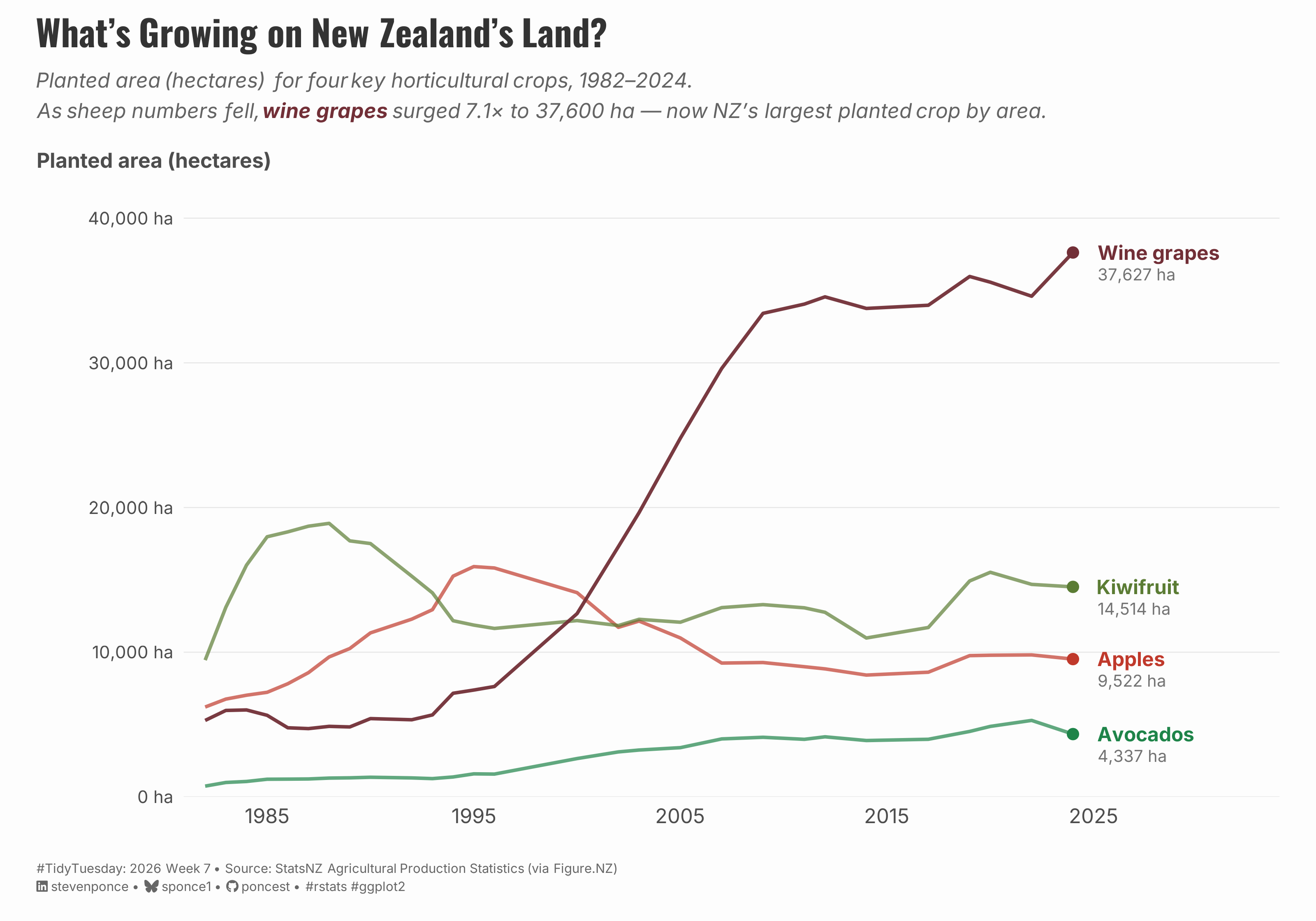
What’s Growing on New Zealand’s Land?

Planted area (hectares) for four key horticultural crops, 1982–2024.

A TidyTuesday visualization exploring New Zealand’s horticultural transformation using StatsNZ agricultural production data. Wine grapes surged 7× to an all-time high while kiwifruit, apples, and avocados each followed distinct growth trajectories. Built with R and ggplot2.

Figure 1: Line chart showing planted area in hectares for four New Zealand horticultural crops from 1982 to 2024. Wine grapes grew dramatically from 5,300 to 37,600 hectares, becoming the largest planted crop. Kiwifruit peaked in the late 1980s, then declined, only partially recovering to 14,500 hectares. Apples peaked in the mid-1990s and settled around 9,500 hectares. Avocados grew steadily from near zero to 4,300 hectares.

Steps to Create this Graphic

1. Load Packages & Setup

```{r}
#| label: load
#| warning: false
#| message: false
#| results: "hide"

## 1. LOAD PACKAGES & SETUP ----
suppressPackageStartupMessages({
if (!require("pacman")) install.packages("pacman")
pacman::p_load(
    tidyverse, ggtext, showtext, janitor, 
    scales, glue
)
})

### |- figure size ----
camcorder::gg_record(
  dir    = here::here("temp_plots"),
  device = "png",
  width  = 10,
  height = 7,
  units  = "in",
  dpi    = 320
)

# Source utility functions
suppressMessages(source(here::here("R/utils/fonts.R")))
source(here::here("R/utils/social_icons.R"))
source(here::here("R/utils/image_utils.R"))
source(here::here("R/themes/base_theme.R"))
```

2. Read in the Data

```{r}
#| label: read
#| include: true
#| eval: true
#| warning: false

tt <- tidytuesdayR::tt_load(2026, week = 07)
dataset_raw <- tt$dataset |> clean_names()
rm(tt)
```

3. Examine the Data

```{r}
#| label: examine
#| include: true
#| eval: true
#| results: 'hide'
#| warning: false

glimpse(dataset_raw)
```

4. Tidy Data

```{r}
#| label: tidy
#| warning: false

### |- filter horticulture crops ----
hort_crops <- c("Wine grapes", "Kiwifruit", "Apples", "Avocados")

hort_data <- dataset_raw |>
  filter(measure %in% hort_crops) |>
  select(
    year = year_ended_june,
    crop = measure,
    hectares = value
  ) |>
  arrange(crop, year) |> 
  mutate(is_focus = crop == "Wine grapes")

### |- calculate growth metrics (robust) ----
hort_growth <- hort_data |>
  group_by(crop) |>
  summarise(
    first_year = min(year),
    last_year = max(year),
    first_value = hectares[year == min(year)] |> first(),
    last_value = hectares[year == max(year)] |> first(),
    peak_value = max(hectares, na.rm = TRUE),
    peak_year = year[which.max(hectares)] |> first(),
    growth_pct = (last_value - first_value) / first_value * 100,
    .groups = "drop"
  )

### |- end-point labels ----
end_labels <- hort_data |>
  group_by(crop) |>
  filter(year == max(year)) |>
  ungroup()

### |- crop-specific label offsets ----
label_offsets <- tibble(
  crop = hort_crops,
  dy   = c(0, 0, -1100, 0) 
)

end_labels2 <- end_labels |>
  left_join(label_offsets, by = "crop") |>
  mutate(dy = replace_na(dy, 0))

### |- compute subtitle stats from data  ----
wine_stats <- hort_growth |>
  filter(crop == "Wine grapes") |>
  mutate(
    last_value_round = round(last_value, -2),
    growth_x         = last_value / first_value
  )

wine_growth_x <- round(wine_stats$growth_x, 1)
wine_last_ha <- comma(wine_stats$last_value_round)
```

5. Visualization Parameters

```{r}
#| label: params
#| include: true
#| warning: false

### |-  plot aesthetics ----
colors <- get_theme_colors(
  palette = c(
      "Wine grapes" = "#722F37",
      "Kiwifruit"   = "#5B7C34",
      "Apples"      = "#C0392B",
      "Avocados"    = "#1E8449"
    )
)

### |- titles and caption ----
title_text <- str_glue("What's Growing on New Zealand's Land?")

subtitle_text <- str_glue(
    "Planted area (hectares) for four key horticultural crops, 1982–2024.<br>",
    "As sheep numbers fell, <b style='color:{colors$palette[\"Wine grapes\"]}'>wine grapes</b> surged ",
    "{wine_growth_x}× to {wine_last_ha} ha — now NZ’s largest planted crop by area."
)

caption_text <- create_social_caption(
    tt_year     = 2026,
    tt_week     = 07,
    source_text = "StatsNZ Agricultural Production Statistics (via Figure.NZ)"
)

### |-  fonts ----
setup_fonts()
fonts <- get_font_families()

### |-  plot theme ----
# Start with base theme
base_theme <- create_base_theme(colors)

# Add weekly-specific theme elements
weekly_theme <- extend_weekly_theme(
  base_theme,
  theme(
    # Text styling
    plot.title = element_text(
      face = "bold", family = fonts$title, size = rel(1.3),
      color = colors$title, margin = margin(b = 10), hjust = 0
    ),
    plot.subtitle = element_markdown(
      face = "italic", family = fonts$subtitle, lineheight = 1.2,
      color = colors$subtitle, size = rel(0.8), margin = margin(b = 20), hjust = 0
    ),

    # Grid
    panel.grid.minor = element_blank(),
    panel.grid.major.x = element_blank(),
    panel.grid.major = element_line(color = "gray90", linewidth = 0.25),

    # Axes
    axis.title = element_text(size = rel(0.8), color = "gray30"),
    axis.text = element_text(color = "gray30"),
    axis.text.y = element_text(size = rel(0.85)),
    axis.ticks = element_blank(),

    # Facets
    strip.background = element_rect(fill = "gray95", color = NA),
    strip.text = element_text(
      face = "bold",
      color = "gray20",
      size = rel(0.9),
      margin = margin(t = 6, b = 4)
    ),
    panel.spacing = unit(1.5, "lines"),

    # Legend elements
    legend.position = "plot",
    legend.title = element_text(
      family = fonts$subtitle,
      color = colors$text, size = rel(0.8), face = "bold"
    ),
    legend.text = element_text(
      family = fonts$tsubtitle,
      color = colors$text, size = rel(0.7)
    ),
    legend.margin = margin(t = 15),

    # Plot margin
    plot.margin = margin(10, 20, 10, 20),
    
  )
)

# Set theme
theme_set(weekly_theme)
```

6. Plot

```{r}
#| label: plot
#| warning: false

### |- final plot ----
p <- ggplot(hort_data, aes(x = year, y = hectares, color = crop)) +

  # Geoms
  geom_line(
    aes(alpha = is_focus),
    linewidth = 0.9
  ) +
  geom_point(
    data = end_labels2,
    size = 2.5, 
    alpha = 1
  ) +
  geom_text(
    data = end_labels2,
    aes(label = crop),
    hjust = 0,
    nudge_x = 1.2,
    size = 3.8,
    fontface = "bold",
    family = fonts$text,
    alpha = 1
  ) +
  geom_text(
    data = end_labels,
    aes(label = glue("{comma(hectares)} ha")),
    hjust = 0,
    nudge_x = 1.2,
    nudge_y = -1500,
    size = 3.2,
    color = "gray45",
    family = fonts$text,
    alpha = 1
  ) +
  # Scales
  scale_color_manual(values = colors$palette) +
  scale_alpha_manual(
    values = c(`TRUE` = 0.95, `FALSE` = 0.70),
    guide = "none"
  ) +
  scale_x_continuous(
    breaks = seq(1985, 2025, 10),
    limits = c(1982, 2034),
    expand = expansion(mult = c(0.02, 0))
  ) +
  scale_y_continuous(
    labels = label_comma(suffix = " ha"),
    breaks = seq(0, 40000, 10000),
    limits = c(0, 42000),
    expand = expansion(mult = c(0, 0.02))
  ) +
  # Labs
  labs(
    title = title_text,
    subtitle = subtitle_text,
    x = NULL,
    y = "Planted area (hectares)",
    caption = caption_text
  ) +
  # Theme
  theme(
    axis.title.y = element_text(
      angle = 0,
      vjust = 1.04,
      hjust = 0.5,
      margin = margin(r = -100)
    ),
    plot.title = element_markdown(
      size = rel(1.4),
      family = fonts$title,
      face = "bold",
      color = colors$title,
      lineheight = 1.15,
      margin = margin(t = 0, b = 5)
    ),
    plot.subtitle = element_markdown(
      size = rel(0.8),
      family = fonts$subtitle,
      color = alpha(colors$subtitle, 0.88),
      lineheight = 1.5,
      margin = margin(t = 5, b = 30)
    ),
    plot.caption = element_markdown(
      size = rel(0.5),
      family = fonts$subtitle,
      color = colors$caption,
      hjust = 0,
      lineheight = 1.4,
      margin = margin(t = 20, b = 5)
    )
  )
```

7. Save

```{r}
#| label: save
#| warning: false

### |-  plot image ----  
save_plot(
  plot = p, 
  type = "tidytuesday", 
  year = 2026, 
  week = 07, 
  width  = 10,
  height = 7,
  )
```

8. Session Info

TipExpand for Session Info

R version 4.4.1 (2024-06-14 ucrt)
Platform: x86_64-w64-mingw32/x64
Running under: Windows 11 x64 (build 26100)

Matrix products: default


locale:
[1] LC_COLLATE=English_United States.utf8 
[2] LC_CTYPE=English_United States.utf8   
[3] LC_MONETARY=English_United States.utf8
[4] LC_NUMERIC=C                          
[5] LC_TIME=English_United States.utf8    

time zone: America/New_York
tzcode source: internal

attached base packages:
[1] stats     graphics  grDevices utils     datasets  methods   base     

other attached packages:
 [1] here_1.0.2      glue_1.8.0      scales_1.4.0    janitor_2.2.1  
 [5] showtext_0.9-7  showtextdb_3.0  sysfonts_0.8.9  ggtext_0.1.2   
 [9] lubridate_1.9.5 forcats_1.0.0   stringr_1.5.1   dplyr_1.1.4    
[13] purrr_1.0.2     readr_2.1.5     tidyr_1.3.1     tibble_3.2.1   
[17] ggplot2_3.5.1   tidyverse_2.0.0 pacman_0.5.1   

loaded via a namespace (and not attached):
 [1] gtable_0.3.6       xfun_0.47          httr2_1.0.1        htmlwidgets_1.6.4 
 [5] gh_1.4.1           tzdb_0.5.0         vctrs_0.6.5        tools_4.4.0       
 [9] generics_0.1.3     parallel_4.4.0     curl_5.2.1         gifski_1.12.0-2   
[13] fansi_1.0.6        pkgconfig_2.0.3    RColorBrewer_1.1-3 lifecycle_1.0.4   
[17] compiler_4.4.0     farver_2.1.2       textshaping_0.3.7  codetools_0.2-20  
[21] snakecase_0.11.1   htmltools_0.5.8.1  yaml_2.3.10        crayon_1.5.2      
[25] pillar_1.9.0       camcorder_0.1.0    magick_2.8.3       commonmark_1.9.1  
[29] tidyselect_1.2.1   digest_0.6.37      stringi_1.8.3      rsvg_2.6.0        
[33] rprojroot_2.1.1    fastmap_1.2.0      grid_4.4.0         cli_3.6.5         
[37] magrittr_2.0.3     utf8_1.2.4         withr_3.0.1        rappdirs_0.3.3    
[41] bit64_4.0.5        timechange_0.4.0   rmarkdown_2.28     tidytuesdayR_1.2.1
[45] gitcreds_0.1.2     bit_4.0.5          ragg_1.3.0         hms_1.1.3         
[49] evaluate_1.0.0     knitr_1.48         markdown_1.12      rlang_1.1.7       
[53] gridtext_0.1.5     Rcpp_1.0.13        xml2_1.3.6         svglite_2.1.3     
[57] rstudioapi_0.16.0  vroom_1.6.5        jsonlite_1.8.9     R6_2.5.1          
[61] systemfonts_1.1.0 

9. GitHub Repository

TipExpand for GitHub Repo

The complete code for this analysis is available in tt_2026_07.qmd.

For the full repository, click here.

10. References

TipExpand for References

1. Data Source:
   • TidyTuesday 2026 Week 07: Agricultural Production Statistics in New Zealand

11. Custom Functions Documentation

Note📦 Custom Helper Functions

This analysis uses custom functions from my personal module library for efficiency and consistency across projects.

Functions Used:

• fonts.R: setup_fonts(), get_font_families() - Font management with showtext
• social_icons.R: create_social_caption() - Generates formatted social media captions
• image_utils.R: save_plot() - Consistent plot saving with naming conventions
• base_theme.R: create_base_theme(), extend_weekly_theme(), get_theme_colors() - Custom ggplot2 themes

Why custom functions?
These utilities standardize theming, fonts, and output across all my data visualizations. The core analysis (data tidying and visualization logic) uses only standard tidyverse packages.

Source Code:
View all custom functions → GitHub: R/utils