More Than Money: How Science Foundation Ireland Built a National Research Ecosystem

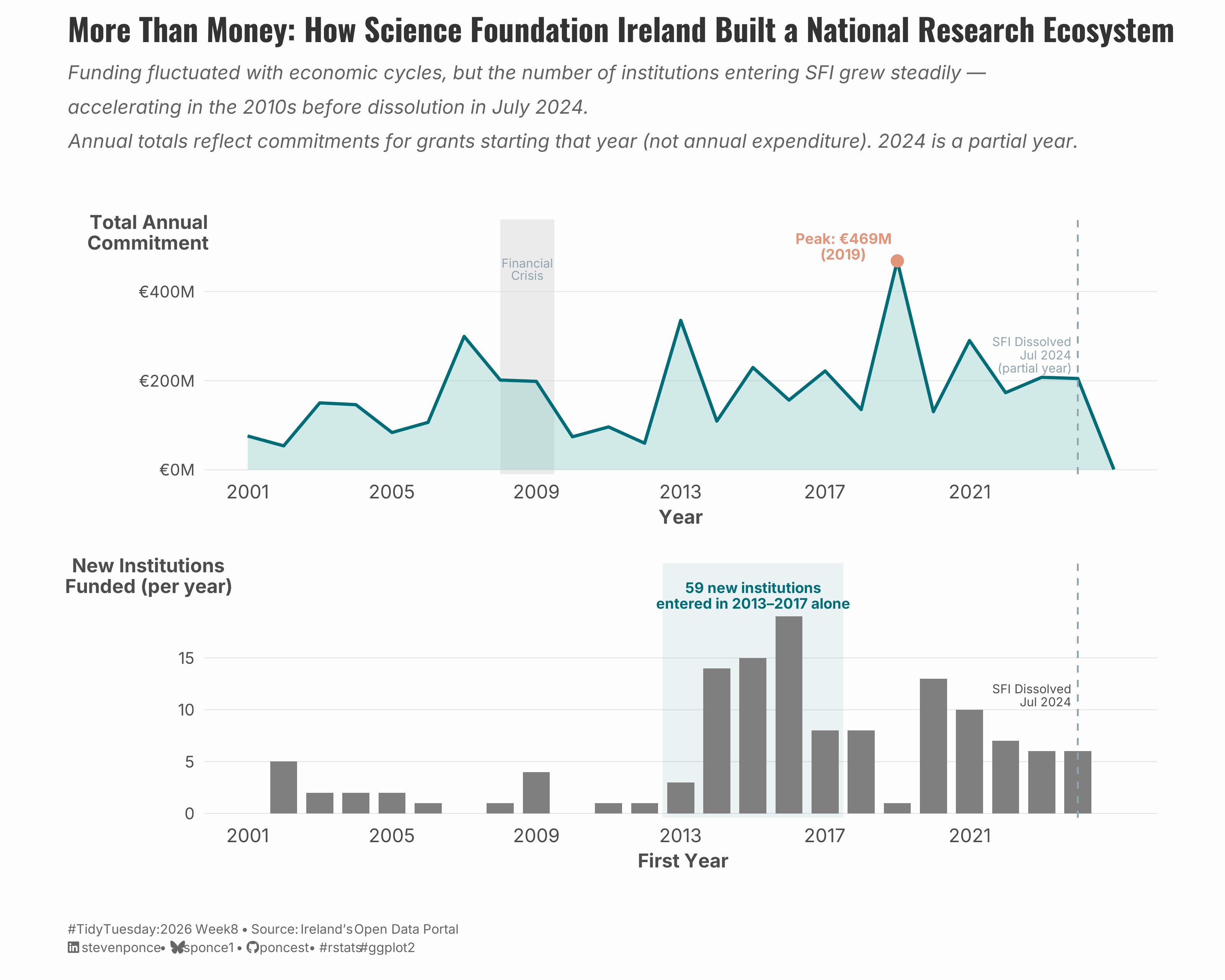
Funding fluctuated with economic cycles, but the number of institutions entering SFI grew steadily — accelerating in the 2010s before dissolution in July 2024.

A two-panel time series examining Science Foundation Ireland’s 24-year legacy (2001–2024). While annual grant commitments fluctuated with economic cycles — peaking at €469M in 2019 — the number of institutions entering the SFI ecosystem grew steadily, with 59 new institutions joining in 2013–2017 alone.

Figure 1: A two-panel time series (2001–2024) exploring Science Foundation Ireland’s legacy. The top panel shows annual grant commitments as a teal area chart, peaking at €469M in 2019 before a sharp 2024 drop reflecting SFI’s July dissolution. The bottom panel shows new institutions funded each year as a bar chart, with 2013–2017 highlighted in teal, during which 59 new institutions entered the ecosystem. Together, the panels argue that while SFI’s funding fluctuated, its institutional reach grew steadily until the end. Note: totals reflect commitments by grant start year, not annual expenditure; 2024 is a partial year.

Steps to Create this Graphic

1. Load Packages & Setup

```{r}
#| label: load
#| warning: false
#| message: false
#| results: "hide"

## 1. LOAD PACKAGES & SETUP ----
suppressPackageStartupMessages({
if (!require("pacman")) install.packages("pacman")
pacman::p_load(
    tidyverse, ggtext, showtext, janitor, 
    scales, glue, patchwork
)
})

### |- figure size ----
camcorder::gg_record(
  dir    = here::here("temp_plots"),
  device = "png",
  width  = 10,
  height = 8,
  units  = "in",
  dpi    = 320
)

# Source utility functions
suppressMessages(source(here::here("R/utils/fonts.R")))
source(here::here("R/utils/social_icons.R"))
source(here::here("R/utils/image_utils.R"))
source(here::here("R/themes/base_theme.R"))
```

2. Read in the Data

```{r}
#| label: read
#| include: true
#| eval: true
#| warning: false

tt <- tidytuesdayR::tt_load(2026, week = 08)
sfi_grants_raw <- tt$sfi_grants |> clean_names()
rm(tt)
```

3. Examine the Data

```{r}
#| label: examine
#| include: true
#| eval: true
#| results: 'hide'
#| warning: false

glimpse(sfi_grants_raw)
```

4. Tidy Data

```{r}
#| label: tidy
#| warning: false

### |- base clean ----
sfi <- sfi_grants_raw |>
  filter(
    !is.na(current_total_commitment),
    current_total_commitment > 0,
    !is.na(start_date),
    !is.na(research_body),
    research_body != ""
  ) |>
  mutate(year = lubridate::year(start_date))

### |- Panel 1: annual funding totals ----
annual_funding <- sfi |>
  group_by(year) |>
  summarise(
    total_funding = sum(current_total_commitment, na.rm = TRUE),
    .groups = "drop"
  ) |>
  arrange(year)

peak_year <- annual_funding |> slice_max(total_funding, n = 1)

### |- Panel 2: new institutions per year ----
inst_by_year <- sfi |>
  group_by(research_body) |>
  summarise(first_year = min(year, na.rm = TRUE), .groups = "drop") |>
  count(first_year, name = "new_inst") |>
  arrange(first_year)

# Surge callout stat
surge_total <- inst_by_year |>
  filter(first_year >= 2013, first_year <= 2017) |>
  summarise(n = sum(new_inst)) |>
  pull(n)

total_inst <- sum(inst_by_year$new_inst)
```

5. Visualization Parameters

```{r}
#| label: params
#| include: true
#| warning: false

### |-  plot aesthetics ----
colors <- get_theme_colors(
  palette = c(
      "accent"       = "#006D77",  
      "accent_light" = "#83C5BE",   
      "bar_muted"    = "#CFD8DC",   
      "peak"         = "#E29578",
      "text_light"   = "#90A4AE"
    )
)

### |- titles and caption ----
title_text <- str_glue(
    "More Than Money: How Science Foundation Ireland Built a National Research Ecosystem"
)

subtitle_text <- str_glue(
    "Funding fluctuated with economic cycles, but the number of institutions entering SFI grew steadily \u2014
accelerating in the 2010s before dissolution in July 2024.
Annual totals reflect commitments for grants starting that year (not annual expenditure). 2024 is a partial year."
)

caption_text <- create_social_caption(
    tt_year     = 2026,
    tt_week     = 08,
    source_text = "Ireland's Open Data Portal"
)

### |-  fonts ----
setup_fonts()
fonts <- get_font_families()

### |-  plot theme ----
# Start with base theme
base_theme <- create_base_theme(colors)

# Add weekly-specific theme elements
weekly_theme <- extend_weekly_theme(
  base_theme,
  theme(
    # Text styling
    plot.title = element_text(
      face = "bold", family = fonts$title, size = rel(1.3),
      color = colors$title, margin = margin(b = 10), hjust = 0
    ),
    plot.subtitle = element_text(
      face = "italic", family = fonts$subtitle, lineheight = 1.2,
      color = colors$subtitle, size = rel(0.8), margin = margin(b = 20), hjust = 0
    ),

    # Grid
    panel.grid.minor = element_blank(),
    panel.grid.major.x = element_blank(),
    panel.grid.major = element_line(color = "gray90", linewidth = 0.25),

    # Axes
    axis.title = element_text(size = rel(0.8), color = "gray30"),
    axis.text = element_text(color = "gray30"),
    axis.text.y = element_text(size = rel(0.85)),
    axis.ticks = element_blank(),

    # Facets
    strip.background = element_rect(fill = "gray95", color = NA),
    strip.text = element_text(
      face = "bold",
      color = "gray20",
      size = rel(0.9),
      margin = margin(t = 6, b = 4)
    ),
    panel.spacing = unit(1.5, "lines"),

    # Legend elements
    legend.position = "plot",
    legend.title = element_text(
      family = fonts$subtitle,
      color = colors$text, size = rel(0.8), face = "bold"
    ),
    legend.text = element_text(
      family = fonts$tsubtitle,
      color = colors$text, size = rel(0.7)
    ),
    legend.margin = margin(t = 15),

    # Plot margin
    plot.margin = margin(10, 20, 10, 20),
    
  )
)

# Set theme
theme_set(weekly_theme)
```

6. Plot

```{r}
#| label: plot
#| warning: false

### |- Panel 1: C1 — Annual Funding ----
p1 <- annual_funding |>
  ggplot(aes(x = year, y = total_funding)) +
  # Annotate
  annotate("rect",
    xmin = 2008, xmax = 2009.5,
    ymin = -Inf, ymax = Inf,
    fill = "gray85", alpha = 0.5
  ) +
  annotate("text",
    x = 2008.75, y = max(annual_funding$total_funding) * 0.96,
    label = "Financial\nCrisis",
    size = 2.5, color = colors$palette["text_light"],
    hjust = 0.5, lineheight = 0.85,
    family = fonts$text
  ) +
  # Geom
  geom_area(fill = colors$palette["accent_light"], alpha = 0.35) +
  geom_line(color = colors$palette["accent"], linewidth = 0.9) +
  geom_point(
    data = peak_year,
    aes(x = year, y = total_funding),
    color = colors$palette["peak"],
    size = 3,
    shape = 21,
    fill = colors$palette["peak"],
    stroke = 0.5
  ) +
  geom_text(
    data = peak_year,
    aes(
      x = year,
      y = total_funding,
      label = glue(
        "Peak: {dollar(total_funding, prefix = '\u20ac', suffix = 'M', scale = 1e-6, accuracy = 1)}\n({year})"
      )
    ),
    nudge_y = max(annual_funding$total_funding) * 0.07,
    nudge_x = -1.5,
    size = 3,
    color = colors$palette["peak"],
    fontface = "bold",
    family = fonts$text,
    lineheight = 0.9
  ) +
  geom_vline(
    xintercept = 2024, linetype = "dashed",
    color = colors$palette["text_light"], linewidth = 0.5
  ) +
  annotate("text",
    x = 2023.8, y = max(annual_funding$total_funding) * 0.55,
    label = "SFI Dissolved\nJul 2024\n(partial year)",
    size = 2.5, color = colors$palette["text_light"],
    hjust = 1, lineheight = 0.9,
    family = fonts$text
  ) +
  # Scales
  scale_y_continuous(
    labels = label_dollar(prefix = "\u20ac", suffix = "M", scale = 1e-6, accuracy = 1),
    expand = expansion(mult = c(0.02, 0.12))
  ) +
  scale_x_continuous(breaks = seq(2001, 2024, 4), limits = c(2001, 2025)) +
  # Labs
  labs(
      x = "Year",
      y = "Total Annual\nCommitment"
      ) +
  # Theme
  theme(
    axis.title.y = element_text(
      angle = 0,
      vjust = 1.02,
      hjust = 0.5,
      margin = margin(r = -50)
    )
  )

### |- Panel 2: C18 — New Institutions per Year ----
p2 <- inst_by_year |>
  ggplot(aes(x = first_year, y = new_inst)) +
  # Annotate
  annotate("rect",
    xmin = 2012.5, xmax = 2017.5,
    ymin = -Inf, ymax = Inf,
    fill = colors$palette["accent"], alpha = 0.07
  ) +
  # Geoms
  geom_col(
    aes(fill = first_year >= 2013 & first_year <= 2017),
    width = 0.75,
    show.legend = FALSE
  ) +
  geom_vline(
    xintercept = 2024, linetype = "dashed",
    color = colors$palette["text_light"], linewidth = 0.5
  ) +
  annotate("text",
    x = 2015, y = 21,
    label = glue("{surge_total} new institutions\nentered in 2013\u20132017 alone"),
    hjust = 0.5, size = 3,
    color = colors$palette["accent"],
    fontface = "bold",
    lineheight = 0.9,
    family = fonts$text
  ) +
  annotate("text",
    x = 2023.8, y = max(inst_by_year$new_inst) * 0.6,
    label = "SFI Dissolved\nJul 2024",
    size = 2.5, color = colors$text,
    hjust = 1, lineheight = 0.9,
    family = fonts$text
  ) +
  # Scales
  scale_fill_manual(
    values = c(
      "TRUE" = colors$palette["accent"],
      "FALSE" = colors$palette["bar_muted"]
    )
  ) +
  scale_y_continuous(
    breaks = seq(0, max(inst_by_year$new_inst), 5),
    expand = expansion(mult = c(0.02, 0.15))
  ) +
  scale_x_continuous(breaks = seq(2001, 2024, 4), limits = c(2001, 2025)) +
  # Labs
  labs(
      x = " First Year",
      y = "New Institutions\nFunded (per year)"
      ) +
  # Theme
  theme(
    axis.title.y = element_text(
      angle = 0,
      vjust = 1.02,
      hjust = 0.5,
      margin = margin(r = -50)
    )
  )

### |- Combined Plots ----
combined_plots <- p1 / p2 +
  plot_layout(heights = c(1, 1)) +
  plot_annotation(
    title = title_text,
    subtitle = subtitle_text,
    caption = caption_text,
    theme = theme(
      axis.title.y = element_text(
        angle = 0,
        vjust = 1.04,
        hjust = 0.5,
        margin = margin(r = -100)
      ),
      plot.title = element_text(
        size = rel(1.3),
        family = fonts$title,
        face = "bold",
        color = colors$title,
        lineheight = 1.15,
        margin = margin(t = 0, b = 5)
      ),
      plot.subtitle = element_text(
        size = rel(0.8),
        family = fonts$subtitle,
        color = alpha(colors$subtitle, 0.88),
        lineheight = 1.5,
        margin = margin(t = 5, b = 30)
      ),
      plot.caption = element_markdown(
        size = rel(0.55),
        family = fonts$subtitle,
        color = colors$caption,
        hjust = 0,
        lineheight = 1.4,
        margin = margin(t = 20, b = 5)
      )
    )
  )
```

7. Save

```{r}
#| label: save
#| warning: false

### |-  plot image ----  
save_plot_patchwork(
  plot = combined_plots, 
  type = "tidytuesday", 
  year = 2026, 
  week = 08, 
  width  = 10,
  height = 8,
  )
```

8. Session Info

TipExpand for Session Info

R version 4.4.1 (2024-06-14 ucrt)
Platform: x86_64-w64-mingw32/x64
Running under: Windows 11 x64 (build 26100)

Matrix products: default


locale:
[1] LC_COLLATE=English_United States.utf8 
[2] LC_CTYPE=English_United States.utf8   
[3] LC_MONETARY=English_United States.utf8
[4] LC_NUMERIC=C                          
[5] LC_TIME=English_United States.utf8    

time zone: America/New_York
tzcode source: internal

attached base packages:
[1] stats     graphics  grDevices utils     datasets  methods   base     

other attached packages:
 [1] here_1.0.2      patchwork_1.3.2 glue_1.8.0      scales_1.4.0   
 [5] janitor_2.2.1   showtext_0.9-7  showtextdb_3.0  sysfonts_0.8.9 
 [9] ggtext_0.1.2    lubridate_1.9.5 forcats_1.0.1   stringr_1.6.0  
[13] dplyr_1.2.0     purrr_1.2.1     readr_2.1.6     tidyr_1.3.2    
[17] tibble_3.3.1    ggplot2_4.0.2   tidyverse_2.0.0 pacman_0.5.1   

loaded via a namespace (and not attached):
 [1] gtable_0.3.6       xfun_0.47          httr2_1.0.1        htmlwidgets_1.6.4 
 [5] gh_1.4.1           tzdb_0.5.0         yulab.utils_0.1.7  vctrs_0.7.1       
 [9] tools_4.4.0        generics_0.1.3     parallel_4.4.0     curl_5.2.1        
[13] gifski_1.32.0-2    pkgconfig_2.0.3    ggplotify_0.1.2    RColorBrewer_1.1-3
[17] S7_0.2.1           lifecycle_1.0.5    compiler_4.4.0     farver_2.1.2      
[21] textshaping_0.3.7  codetools_0.2-20   snakecase_0.11.1   htmltools_0.5.8.1 
[25] yaml_2.3.10        crayon_1.5.2       pillar_1.11.1      camcorder_0.1.0   
[29] magick_2.9.0       commonmark_2.0.0   tidyselect_1.2.1   digest_0.6.37     
[33] stringi_1.8.3      labeling_0.4.3     rsvg_2.6.0         rprojroot_2.1.1   
[37] fastmap_1.2.0      grid_4.4.0         cli_3.6.5          magrittr_2.0.4    
[41] withr_3.0.1        rappdirs_0.3.3     bit64_4.0.5        timechange_0.4.0  
[45] rmarkdown_2.28     tidytuesdayR_1.2.1 gitcreds_0.1.2     bit_4.0.5         
[49] hms_1.1.4          evaluate_1.0.0     knitr_1.48         markdown_1.12     
[53] gridGraphics_0.5-1 rlang_1.1.7        gridtext_0.1.5     Rcpp_1.1.1        
[57] xml2_1.5.2         vroom_1.6.5        svglite_2.2.2      rstudioapi_0.18.0 
[61] jsonlite_2.0.0     R6_2.5.1           fs_1.6.4           systemfonts_1.3.1 

9. GitHub Repository

TipExpand for GitHub Repo

The complete code for this analysis is available in tt_2026_08.qmd.

For the full repository, click here.

10. References

TipExpand for References

1. Data Source:
   • TidyTuesday 2026 Week 08: Science Foundation Ireland Grants Commitments

11. Custom Functions Documentation

Note📦 Custom Helper Functions

This analysis uses custom functions from my personal module library for efficiency and consistency across projects.

Functions Used:

• fonts.R: setup_fonts(), get_font_families() - Font management with showtext
• social_icons.R: create_social_caption() - Generates formatted social media captions
• image_utils.R: save_plot() - Consistent plot saving with naming conventions
• base_theme.R: create_base_theme(), extend_weekly_theme(), get_theme_colors() - Custom ggplot2 themes

Why custom functions?
These utilities standardize theming, fonts, and output across all my data visualizations. The core analysis (data tidying and visualization logic) uses only standard tidyverse packages.

Source Code:
View all custom functions → GitHub: R/utils